Creating Insect Swarms Using Nuke’s Particle System

⭐ How to build adjustable elements of insect swarms…

Adding Life To A Scene 

Sometimes, a composite (particularly DMP and CG scenes) can look lifeless. 

A nice way to add a touch of life and visual interest to a scene, is to put some insects buzzing around in the background – if and when appropriate.  

You could for example add some moths around a lamppost, some gnats or mosquitoes near a body of water or a swamp, or some flies by a trash bin. 

Just in a subtle way – enough to give the audience a sense that there is life and movement in the shot, but without drawing their eyes to it. 

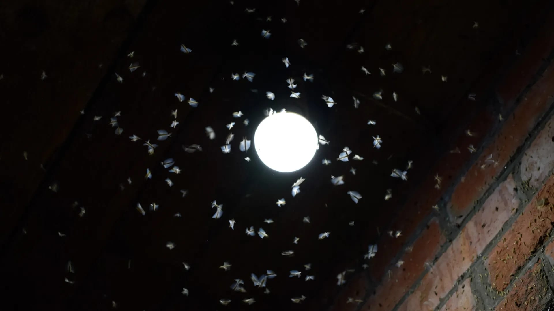
Insects drawn to the light from an outdoor lamp.

Gnats congregating near a beach.

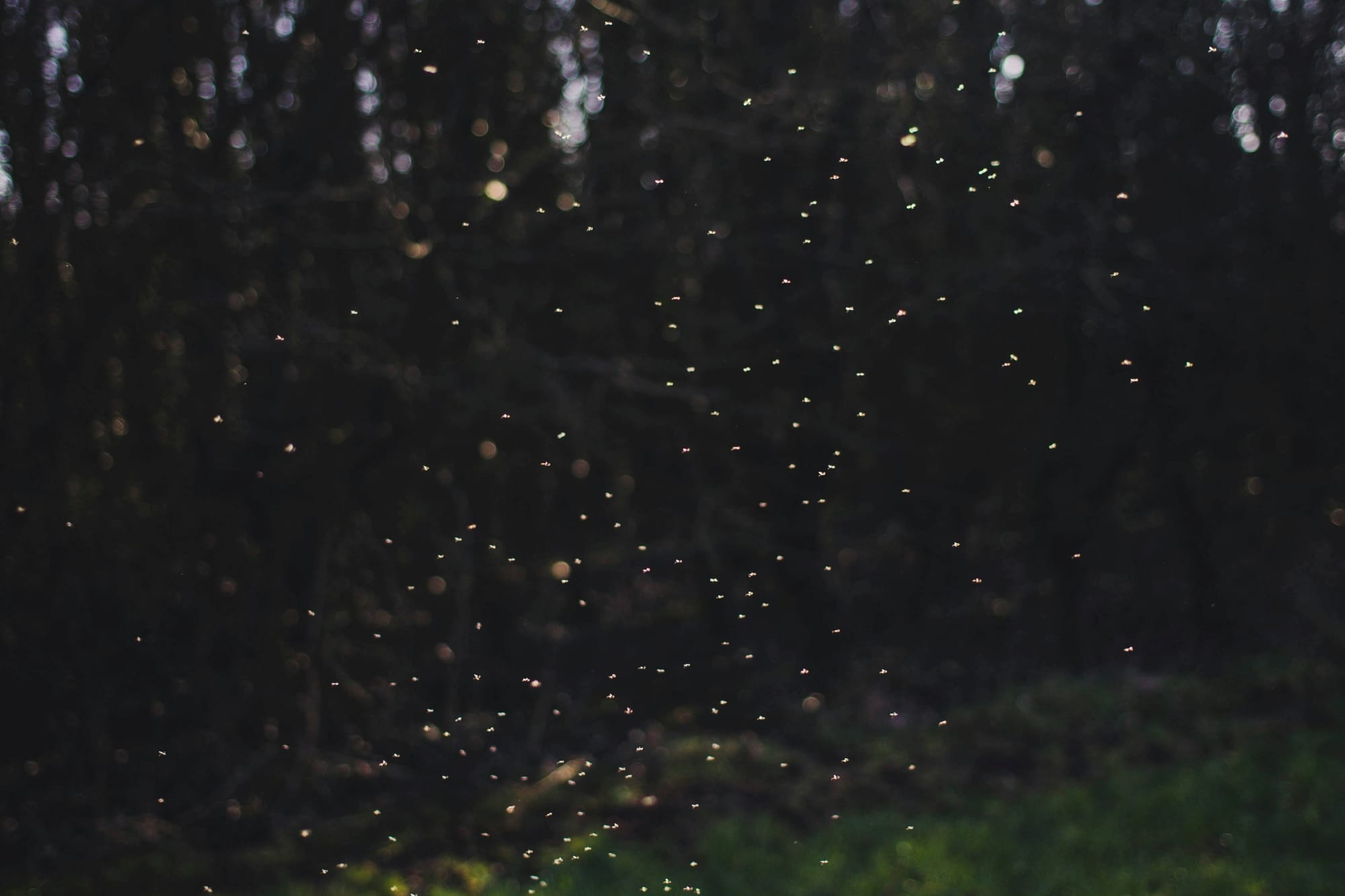
Mayflies in a forest clearing. 

Flying insects, perhaps particularly when in groups, can appear to move erratically – with complex, turbulent flight paths. 

One moment, an insect could be high up in the swarm, and in the next, it’s swooped down below. And, before you know it, it could fly off to the side, and then back up again. – All with a mix of curved, zig zagging, and straight line movement. 

With the exception of wasps which can form an attacking swarm, flying insects typically gather in airborne clusters for mating purposes. (If you’ve ever cycled through a woodland path and gotten a face full of gnats at some point, you’ve likely interrupted an orgy). And this can lead to complex interactions and murmurations. 

In the second image above (i.e. the GIF), we can see that the insects in the swarm are moving quite fast and erratically – rapidly and frequently changing direction. Yet their movements affect one another in a complex chain reaction. And, we can see that there are lots of insects airborne at the same time. 

We can mimic this behaviour with Nuke’s particle system. 

First, let’s create some basic, animated insect geometry to use for our particles. 

Creating The Insect

From a distance, we can’t make out much detail per insect – just a core body shape and two wings which are flapping at a high frequency. 

And that’s really all we need to make. 

First, to build the body, create a Sphere (here called Sphere1) and squash it down to an oval shape like this:

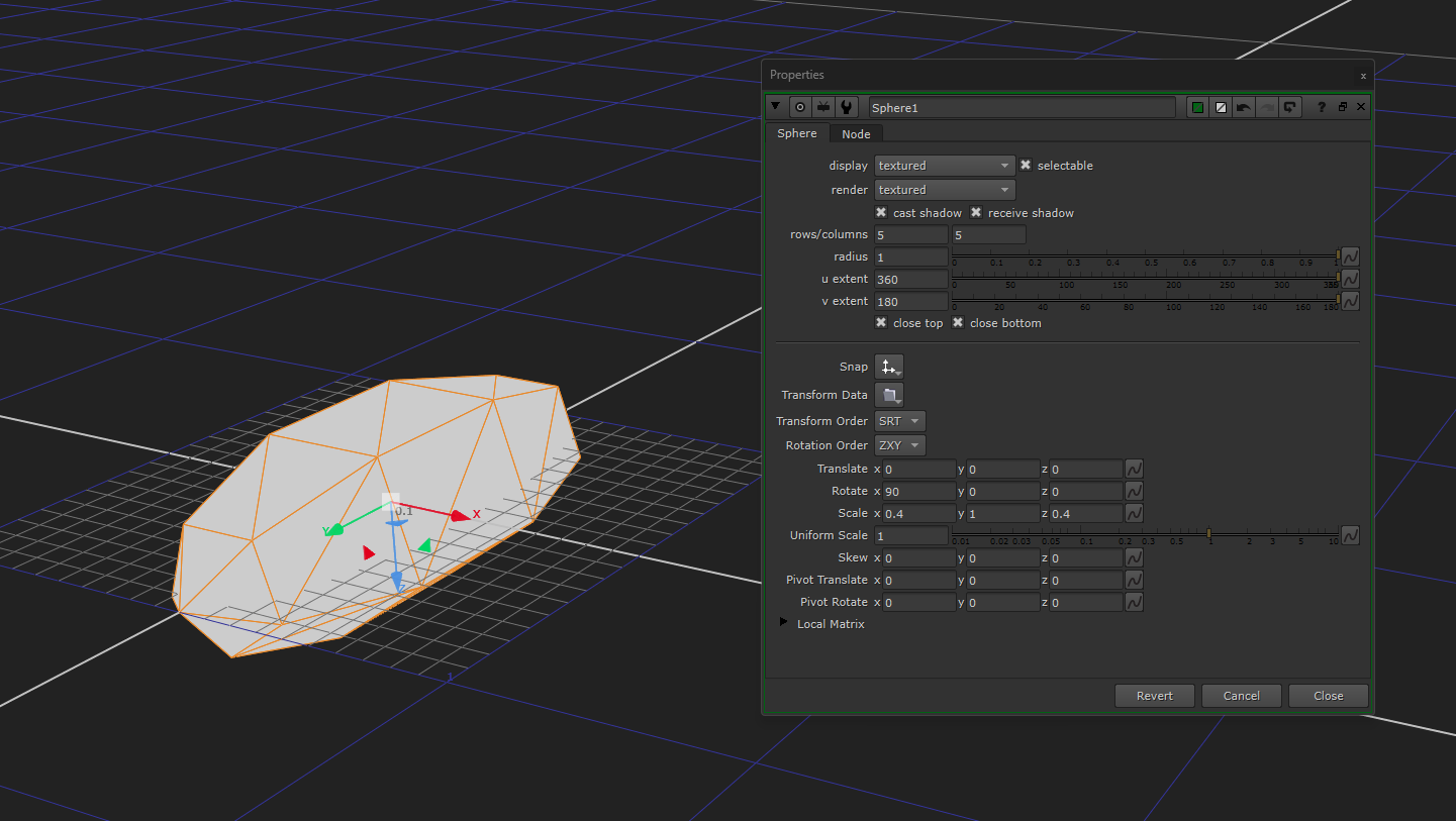
Creating the insect body out of a Sphere. 

Next, to build a wing, create another Sphere (here called Sphere2) and squash it flat like this: 

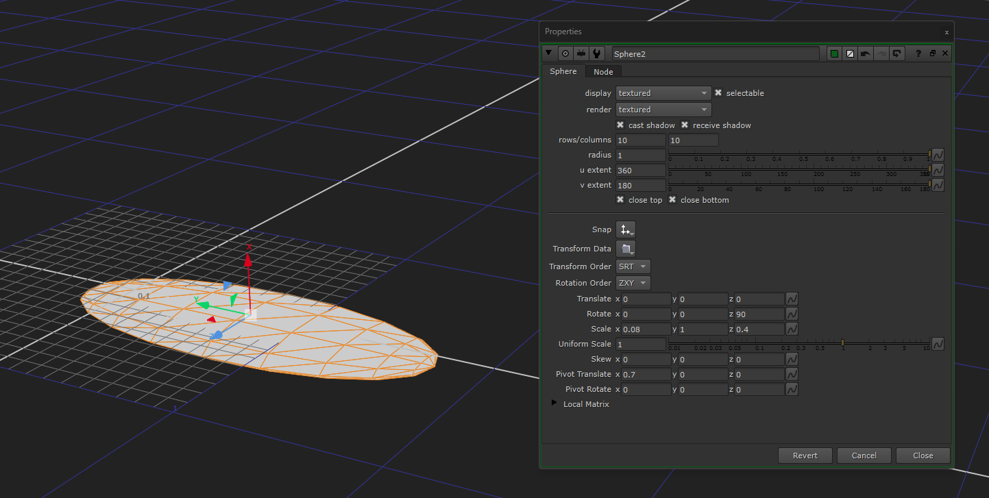
Creating a wing out of a Sphere. 

To make the second wing, simply add a TransformGeo node (here called TransformGeo1) to the first wing (the Sphere2 node), and set it to a scale of -1 in X:

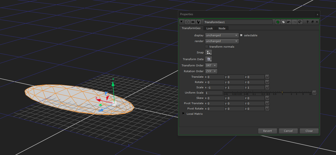
Creating the second wing. 

In order to procedurally animate the wing movement, you can add a second TransformGeo node (TransformGeo2) to the pipe, right after the first wing (the Sphere2 node), with a custom expression in the Z rotation. 

– For a more rhythmic and even flapping of the wings, you can use a sine wave function, and for a more erratic movement you can use a random function. 

So, in the rotate.z knob in the TransformGeo2 node, you can for example add the following expression: 

sin(frame)*60

Or: 

random(1,frame*3)*50

You could even combine the two types of expressions, and have an underlying rhythmic flapping, broken up by some randomness. For example: 

sin(frame)*35 + random(1,frame*3)*40

Change up the values and try out some variations until you find a movement that fits your particular insect type. 

To create a single geometry to use for the particles, merge all three pieces together using a MergeGeo node. 

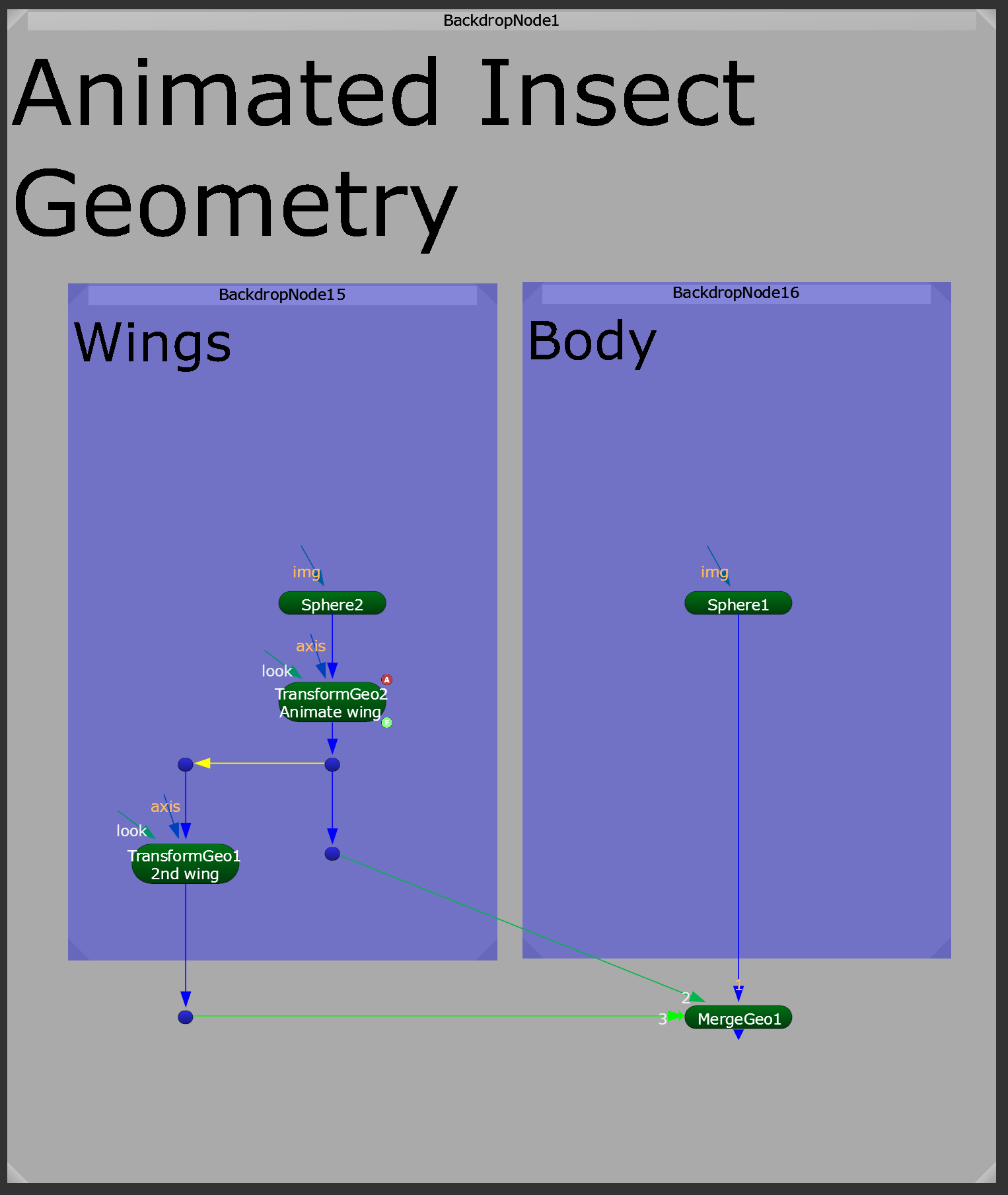
Merging the geometry. 

To help us grade the body and wings separately later on, connect a pure red Constant node to the Sphere1 node (for the insect body), and a pure green Constant node to the Sphere2 node (for the wings). 

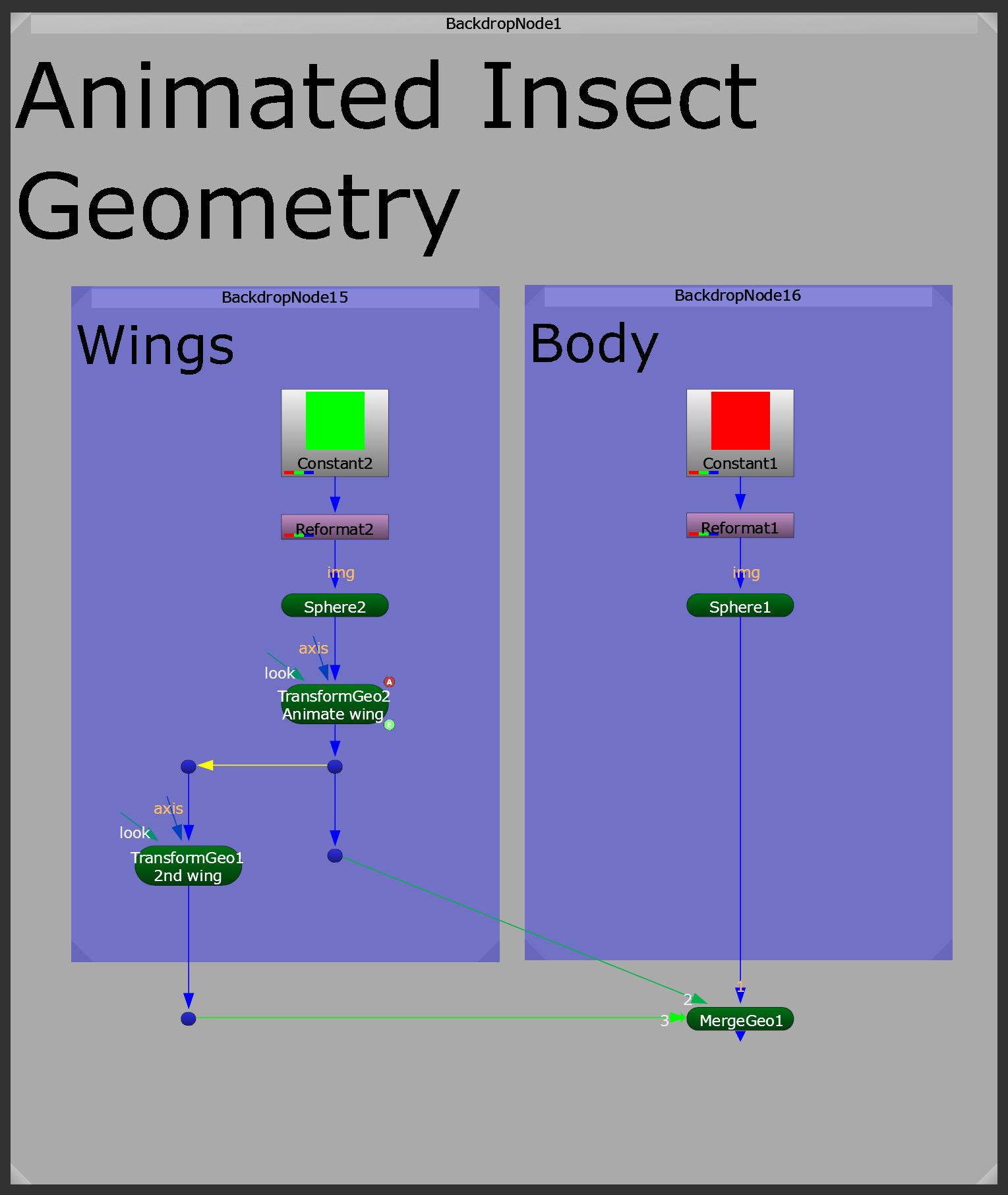
Adding primary colours to the insect geometry. 

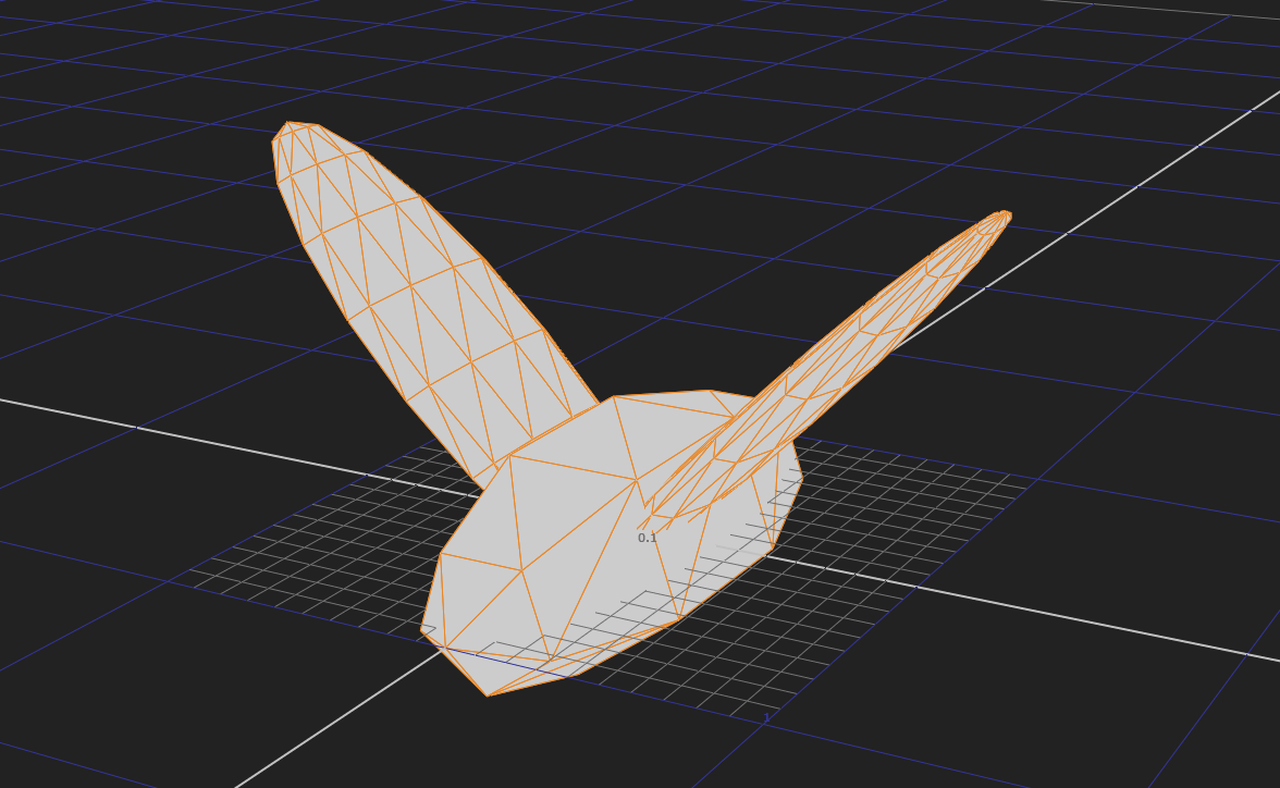
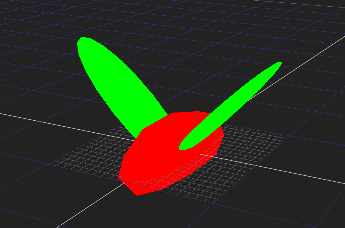
And now, we’ve got animated, ‘textured’ geometry for the particles. 

Animated insect geometry. 

Since we’re animating the wings with an expression, the animation goes on forever, without any specific frame range. To help us later on, let’s add a FrameRange node to our setup, and specify a frame range for our animation. 

It’s often useful to render out over-length insect elements, so that you can time offset them and re-use them across several shots in a sequence. So, let’s set the frame range to something long, for example frame 1-700: 

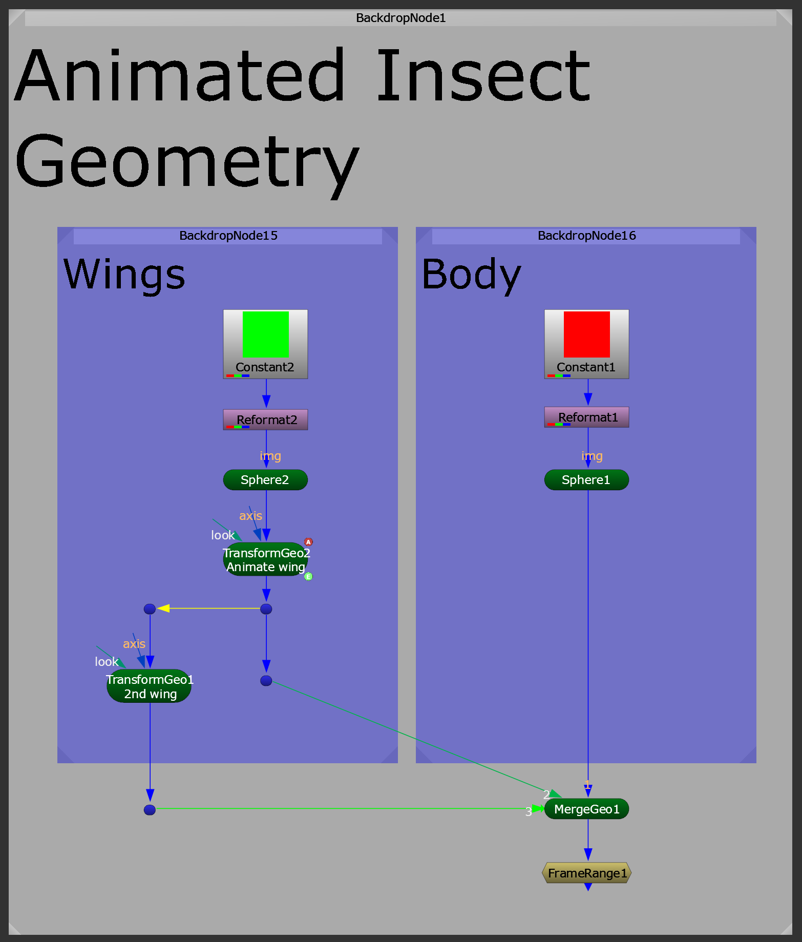
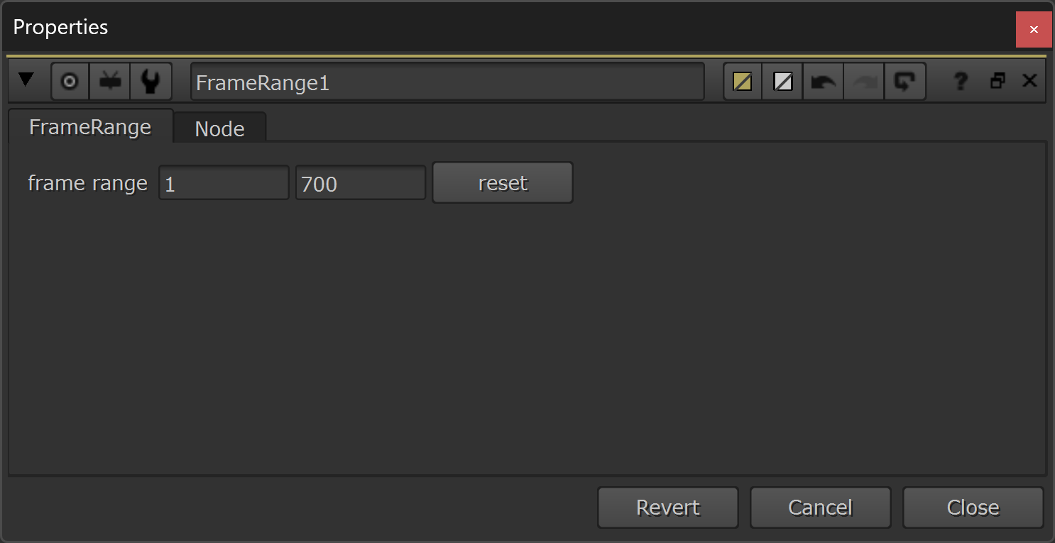
Specifying a frame range for our animation. 

Note that this frame range doesn’t start on the frame that your shot starts on (your shot might for example start on frame 1001) – it only specifies how long the animation should be. In this case, 700 frames. 

Okay, now we’re ready to use the geometry that we’ve made for our particles. 

So let’s create a particle system. 

Emitting The Insects

First, let’s make a shape to emit the particles from. 

For that, we can create another Sphere:

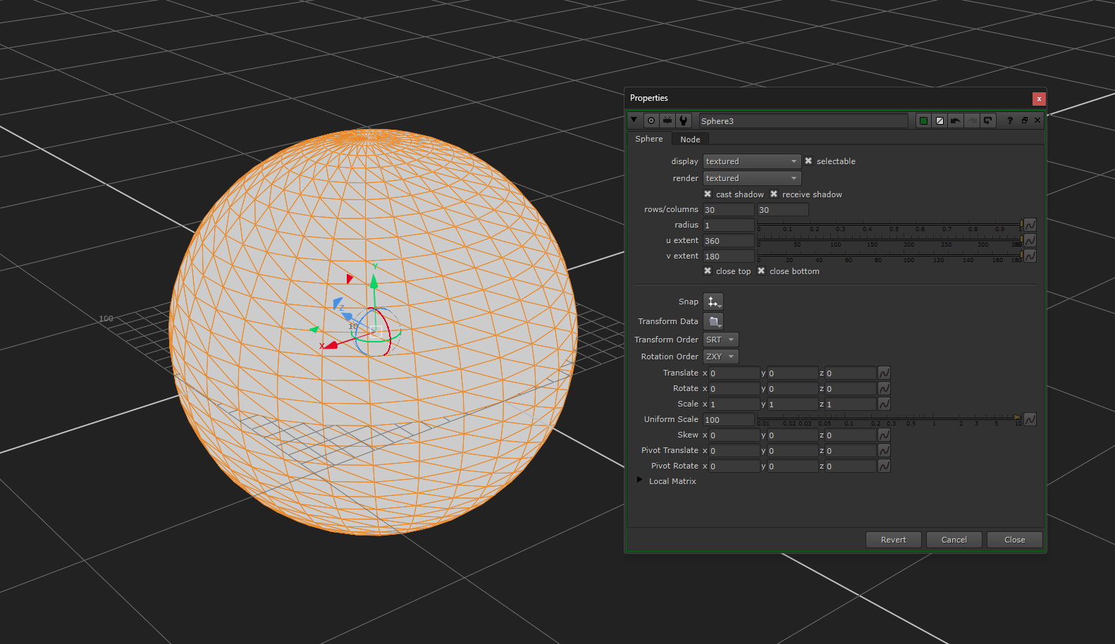
Making a shape to emit the particles from. 

Connect this emitter-geometry and the animated insect-geometry to a ParticleEmitter node’s emit and particle inputs, respectively.

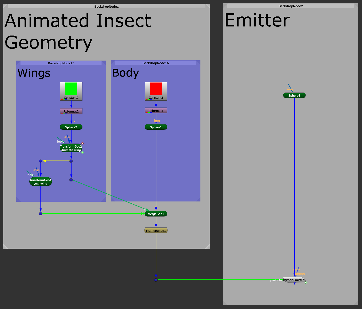
Creating a ParticleEmitter. 

Now, what we want to do is to create a certain number of particles sometime before the first frame of our shot – so that the particles already exist at the start of our shot. And these particles should exist the whole way throughout the length of the shot. 

– We don’t want insects to spawn out of thin air, or suddenly disappear, during our shot. 

So, we have to adjust the start frame of our simulation so that it’s at some frame before the first frame of our shot, and we also have to adjust the particles’ lifetime so that it’s long enough to cover the entire shot. 

Another thing to keep in mind is so-called “pre-roll”. We want the particles to have enough time to spawn, and to get affected by various forces, so that at the beginning of the shot they are already positioned and moving the way we want them to. 

I.e. so that they’re not still being spawned or adjusting into their positions when the shot starts. 

Since frame 1001 is a very common start frame in VFX, I’m going to be using that as our “shot’s” start frame. 

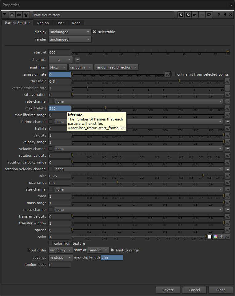
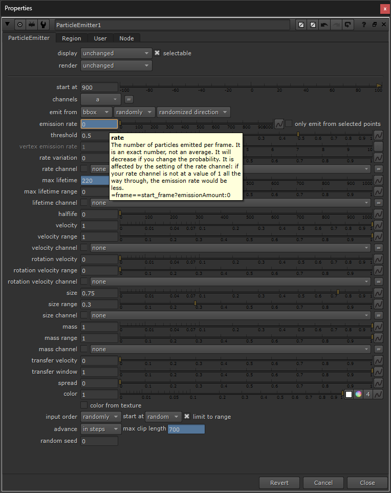
Which means, I’ll set the start frame of the simulation to be well before that, in order to give the simulation enough time to ‘settle’. In this example, I’ll set the start_frame knob in the ParticleEmitter to frame 900. 

Next, to ensure the particles’ lifetime covers the entire length of the shot, I’ll put the following expression into the lifetime knob: 

root.last_frame-start_frame+20

This expression will take the last frame of the shot’s frame range from the project settings, i.e. from the root (root.last_frame), then subtract the simulation’s start frame (start_frame) from it, and then add a 20 frame safety buffer. – Which will ensure that the particles don’t despawn over the course of the shot. 

The lifetime value will now dynamically update for every shot, and so the setup can be copied and reused without worrying about the lifetime of the particles. 

Dynamically setting the particles’ lifetime with an expression. 

We also have to specify when the particles should be spawned, and how many of them should spawn, in the rate knob. 

We could manually animate this, but let’s add an expression here, as well, to make adjusting the number of insects quicker and easier. 

First let’s add a user knob where we can specify the number of particles to spawn. 

Enable the little pen icon at the top of the properties panel, and then drag and drop a Floating Point Slider onto the properties of the ParticleEmitter node. 

Name it for example emissionAmount. Then, disable the pen icon again, and set the value of the emissionAmount knob to for example 200. (An emission rate of 200 simply means that 200 particles will spawn per frame).

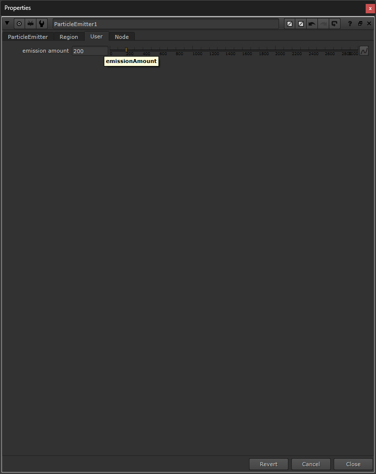
Adding a user knob called emissionAmount. 

Next, in the rate knob of the ParticleEmitter node, add the following expression: 

frame==start_frame?emissionAmount:0

The expression above will spawn the specified number of particles (i.e. the emissionAmount, which is 200) on the simulation's start frame. In this case, that’s on frame 900 (however, the particles will actually show up on the next frame, frame 901). 

Then, it will completely stop spawning any more particles.

Adding an expression to the rate knob for controlling the particle emission. 

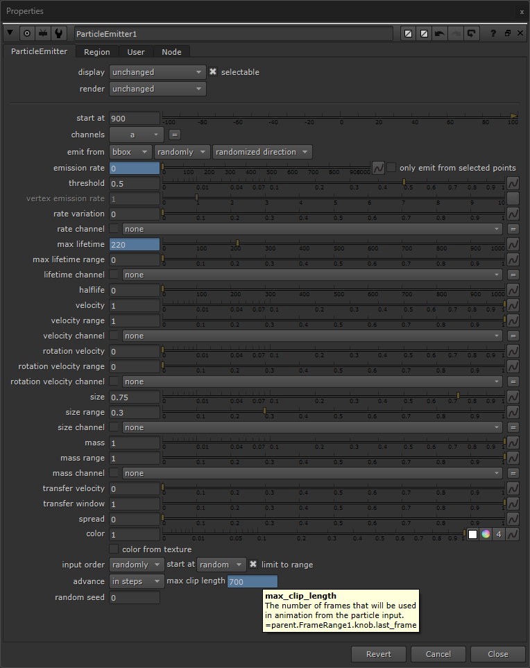
Next, in the ParticleEmitter node, make sure to set the emit from options to: bbox, randomly, and randomized direction, to give our particles a more random movement and spread. 

Then, set the velocity range to 1 to add more variation to the velocity of the particles.

Next, adjust the size and size range to taste. Here, I’ve set them to 0.75 and 0.3, respectively. 

Also change the mass range to 1 to add more variation to the mass of the particles. This will help create more variation in their movement when we apply forces to the particles later on.  

At the bottom of the ParticleEmitter node’s properties, set the input order to randomly, the start at to random, and then tick limit to range. This will make the animation of each insect more randomised, while keeping it within the frame range that we’ve set. 

Lastly, add the following expression to the max clip length knob: 

parent.FrameRange1.knob.last_frame

(Change “FrameRange1” to the name of your FrameRange node, if different). 

This will ensure that the animation doesn’t stop at any point, but that you make use of the full range which you set earlier, e.g. 700 frames. 

Adding an expression to the max clip length. 

Now, we have 200 flying insects nicely spread out, but they are all continuously moving outward. 

The current movement of the insect particles.  

Next, let’s control their movement. 

Adding Forces To The Insects

We want the insects to stay clustered together in a swarm. 

So, first, let’s stop them from constantly drifting further apart like they currently do. 

There are different ways that you could do this. 

You could for example slow down the outward drifting by connecting a ParticleDrag node after the ParticleEmitter node, and increasing the drag value. 

However, to contain the particles with more control, let’s instead connect a ParticlePointForce node after the ParticleEmitter node. 

The ParticlePointForce lets you attract or repel particles to or from a certain point in 3D space. 

Our particles are currently emanating outward from the origin, and so we want to attract them back toward the origin – countering the outward movement. 

By changing the strength value to a negative value, you attract the particles to the point. 

In this case, I set the strength value to -1.65. 

By default, the strength falloff is set to inverse square, but let’s change that to inverse in order to keep a stronger pull further out from the centre, and thus keeping a better hold of our particles. 

And, to actually affect the particles, increase the radius value enough for the effect to encompass them. 

In this case, I set the radius value to 195. 

The position is by default set to the origin (0, 0, 0), so we can leave the x, y, and z values as they are.

The properties of the ParticlePointForce node. 

Countering the outward movement of the insect particles. 

That helps our insects to stay together, but they aren’t moving quite like a swarm yet. 

Let’s introduce more chaotic movement, like we saw in the GIF earlier, by adding some turbulence. 

Connect a couple of ParticleTurbulence nodes after the ParticlePointForce node:

The properties of the first two ParticleTurbulence nodes. 

Above, I have just expression-linked the second and third columns to the first ones, so that I only have to adjust the values in one column, and they’ll update in all three. 

– I.e. in both the strength.y and strength.z knobs, I’ve put the expression strength.x. And so forth. 

In the ParticleTurbulence1 node, I’ve put low-strength, large-scale turbulence values, and in the ParticleTurbulence2 node, I’ve put a little bit higher strength, but small-scale turbulence values. 

This will layer different types of particle movement together and create more variation. 

Next, to push the particles a little bit more away from the origin, let’s add another ParticlePointForce node, this time with a positive strength value:

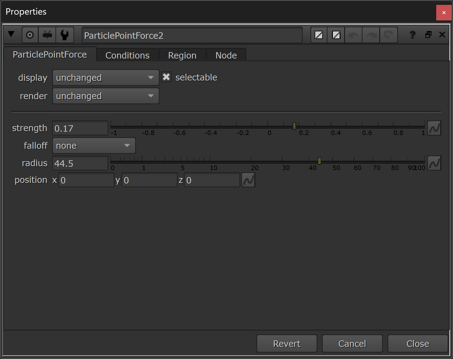
Adding a second ParticlePointForce node. 

This force is just meant to gently push away the particles from the very centre, so both the strength and radius values are quite low: 0.17 and 44.5, respectively. 

Next, let’s add yet another layer of complexity to the movement of the swarm, by adding a third ParticleTurbulence node. This one with a low strength value (0.16) and a high scale value (200):

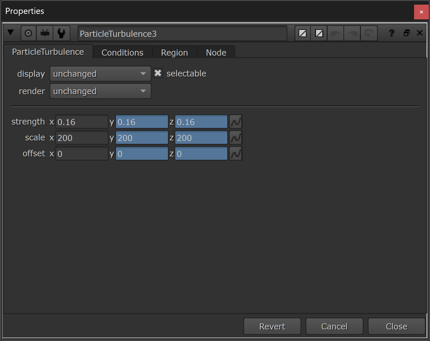
Adding a third ParticleTurbulence node. 

Now, the particles are moving around a bit more randomly – and there is some nice complexity within the swarm: 

Adding turbulence to the insects. 

However, the insects don’t seem to interact with each other too much, yet. 

If you look back at the GIF of the gnats on the beach, there is some subtle murmuration happening there. In all of the chaos, the insects do in fact partly synchronise in moments, and move in a fluid, complex chain reaction. 

We can mimic this murmuration with the ParticleVortex node, which applies a circular force to the particles, attracting them towards an imaginary line. 

Add a couple of ParticleVortex nodes, with the following settings and expressions:

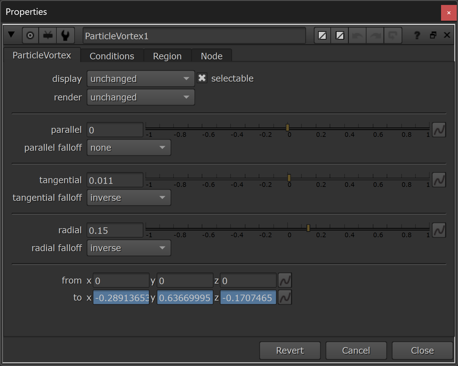
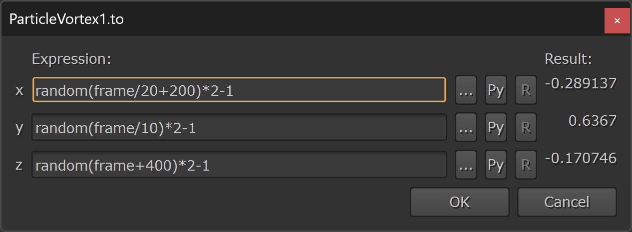
The properties of the ParticleVortex1 node.

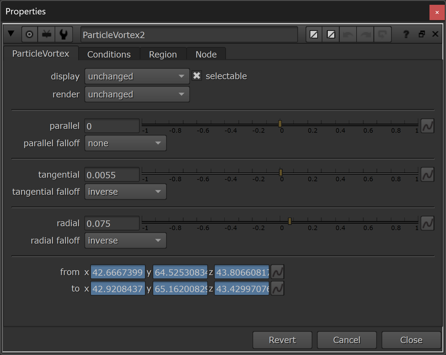
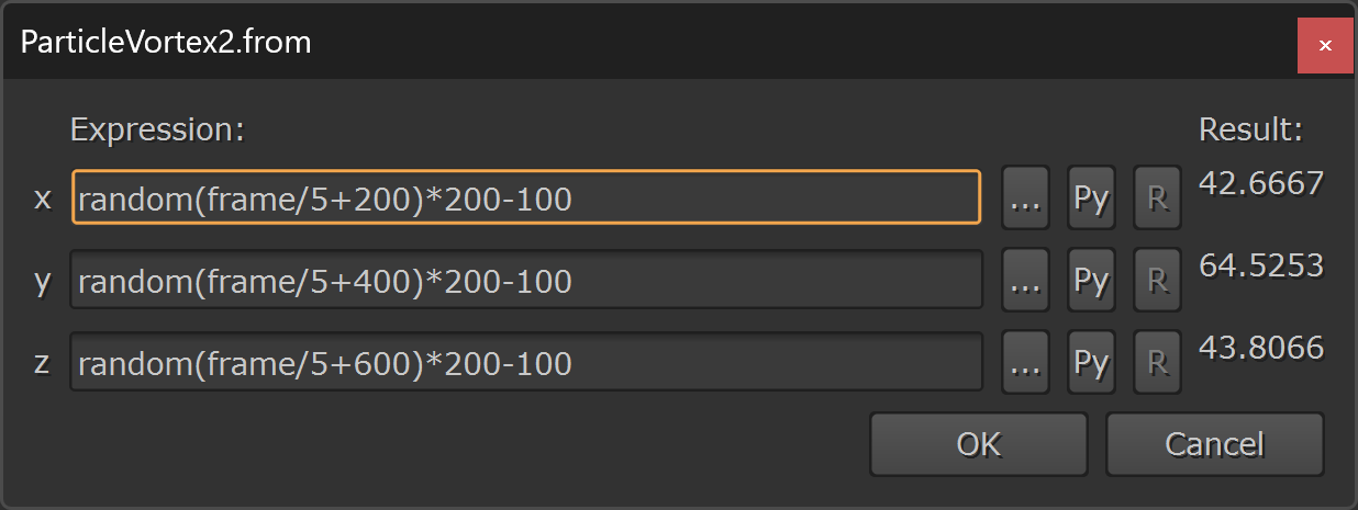
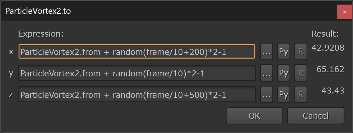
The properties of the ParticleVortex2 node. 

This gives us some more interesting behaviour: 

Creating murmuration in the particles. 

We do see, however, that some of the particles slow down too much at certain times due to the strong forces being applied to them. 

We can counter this slow-down by adding a ParticleSpeedLimit node, and increasing the minimum particle speed:

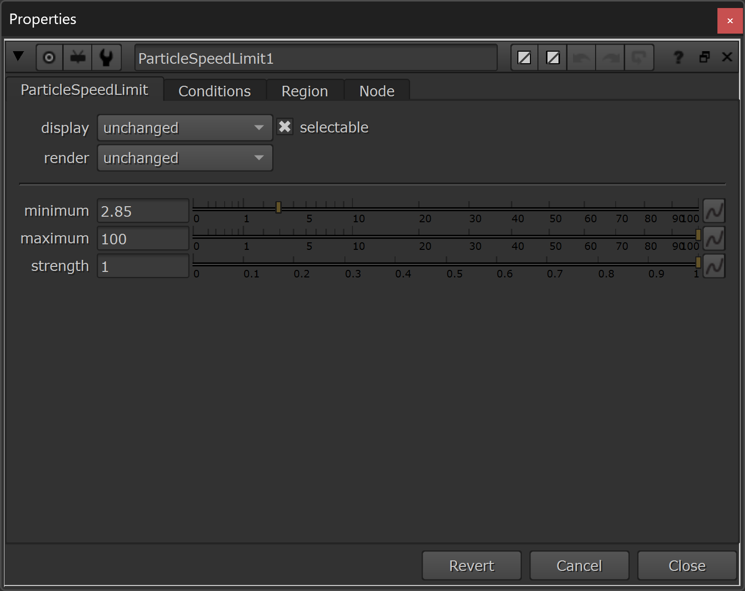
Increasing the minimum particle speed to 2.85. 

The “stickiness” of the murmuration is also still a bit strong, so let’s add another ParticleTurbulence node to break up the particle movement a bit more:

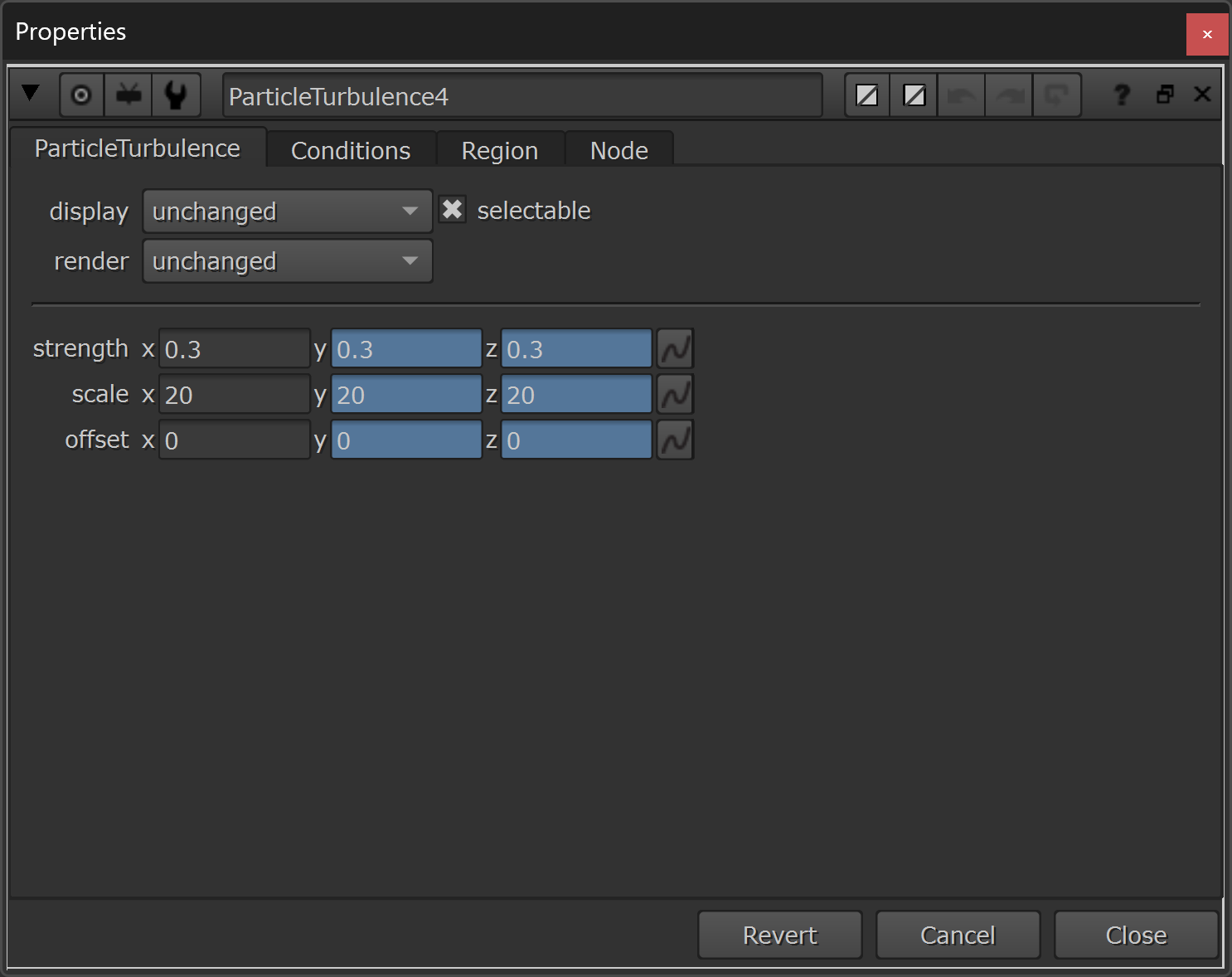
Adding a fourth ParticleTurbulence node. Fairly strong (0.3), but with a low scale (20). 

Finally, we want to make sure that the insects are actually facing the direction that they’re traveling in. 

We can accomplish this by adding a ParticleMotionAlign node, as the last node in our stack of particle forces:

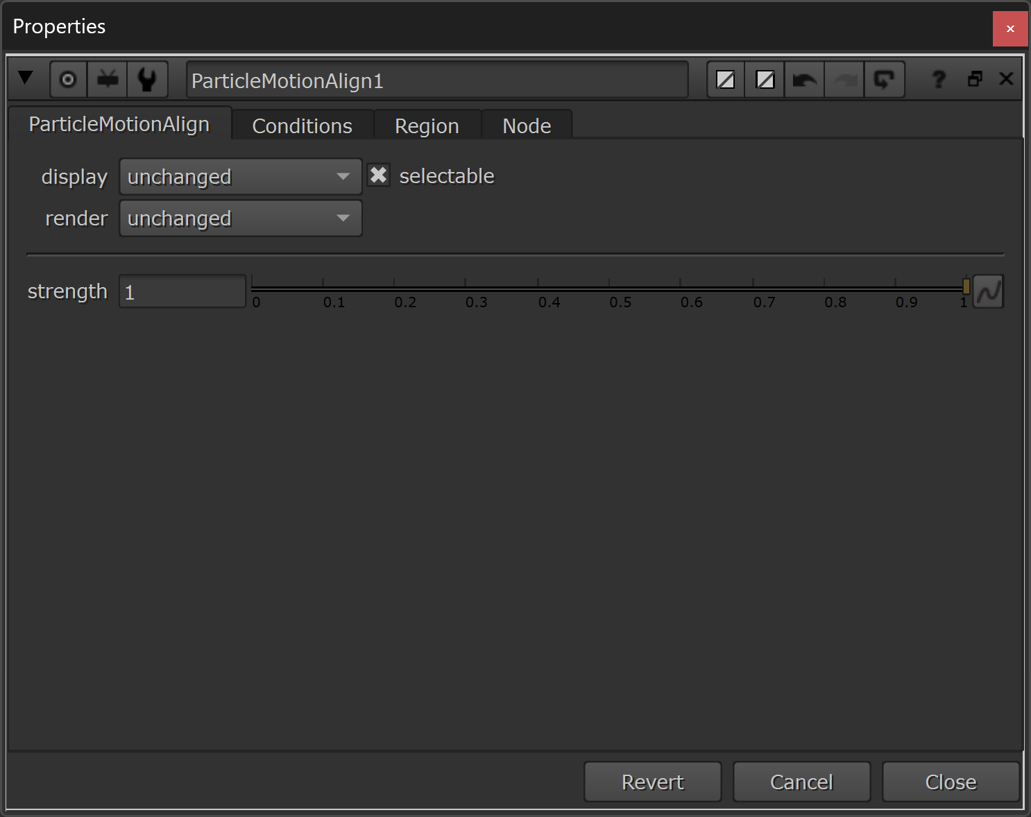
Aligning the particles to their direction of travel. 

The default strength of 1 means that the insects will be completely orientated along their path of travel on each frame, which is what we want.

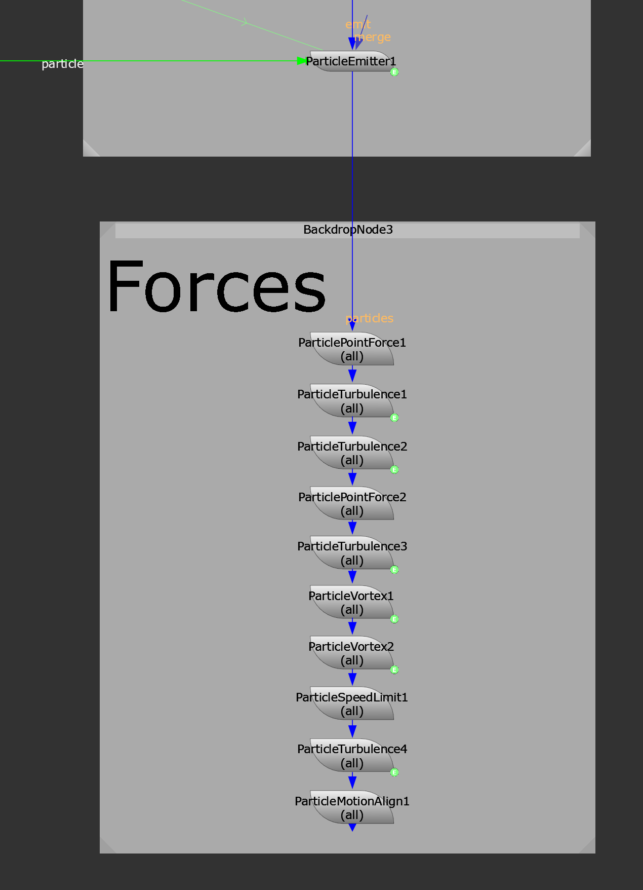
All of the forces applied to the particles. 

Now, we’ve got complex and layered animation, and our insects are behaving in a realistic way: 

All the forces being applied to the particles. 

But they’re still all in 3D space, so let’s output them to a 2D image sequence. 

Outputting The Particles

Connect the last node in the stack of forces (i.e. the ParticleMotionAlign node) and a Camera to a ScanlineRender node. 

In the ScanlineRender node, make sure to output motion vectors, and both normal and position passes:

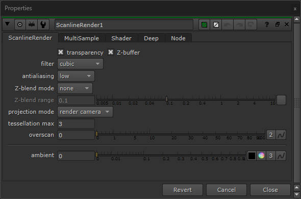
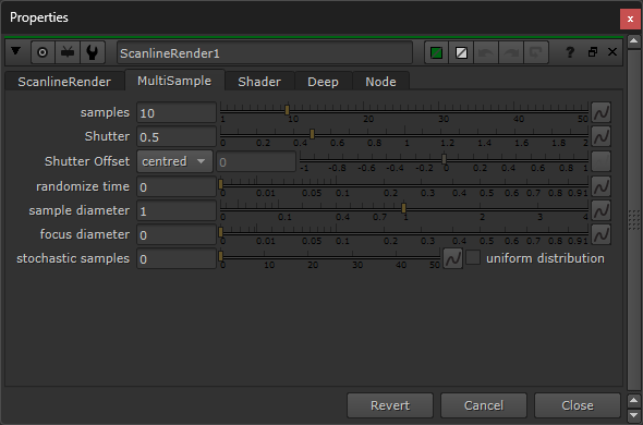
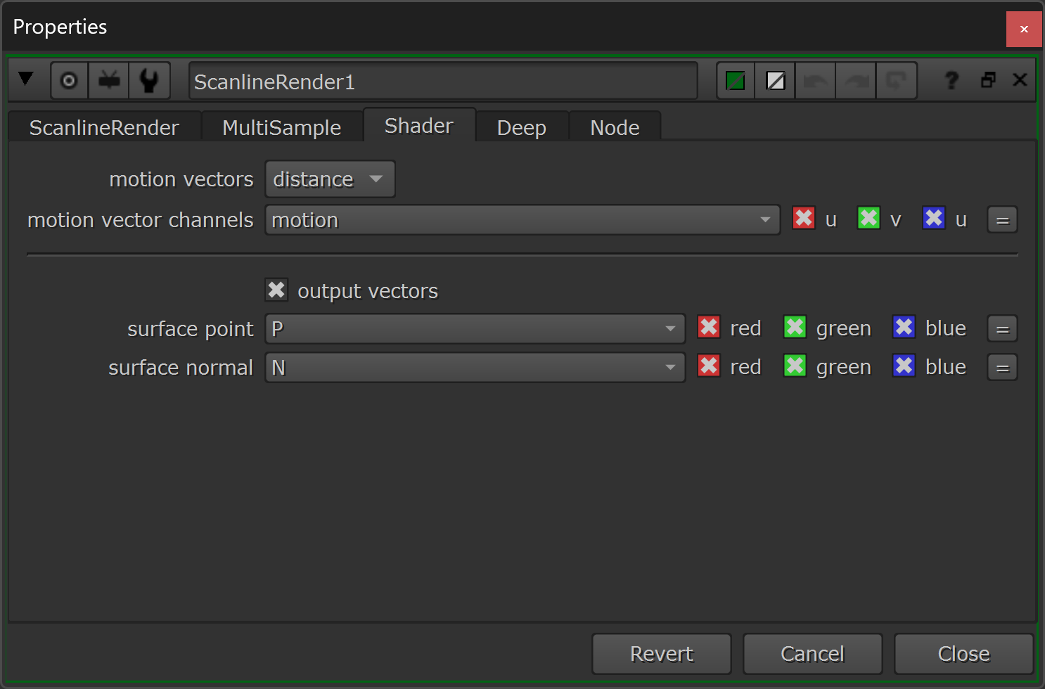
The properties of the ScanlineRender node. 

And, make sure that the Camera is pushed back far enough in Z to capture all of the insects in the frame:

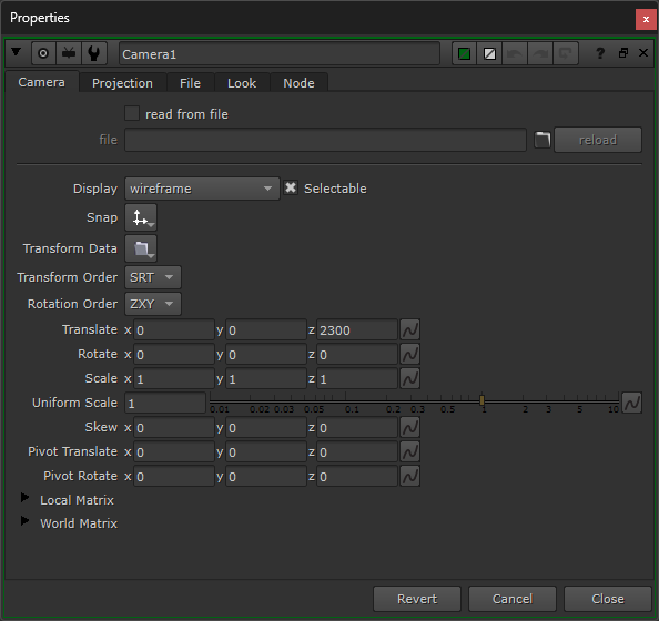
The properties of the Camera. (Translate.z = 2300). 

That way, you can render elements of insects without them breaking the frame. 

The next steps are optional, depending on how you work: 

The ScanlineRender node outputs the additional AOVs unpremultiplied, and the depth.z channel is also inverted, i.e. the depth values are not the real distances to the object, but 1/distance. 

We can premultiply each individual AOV using Premult nodes. And, for the depth.z channel, we can combine the premultiplication and the depth inversion, by connecting an Expression node with the following expression in the depth.z channel: 

depth.Z == 0 ? 0 : 1/depth.Z*a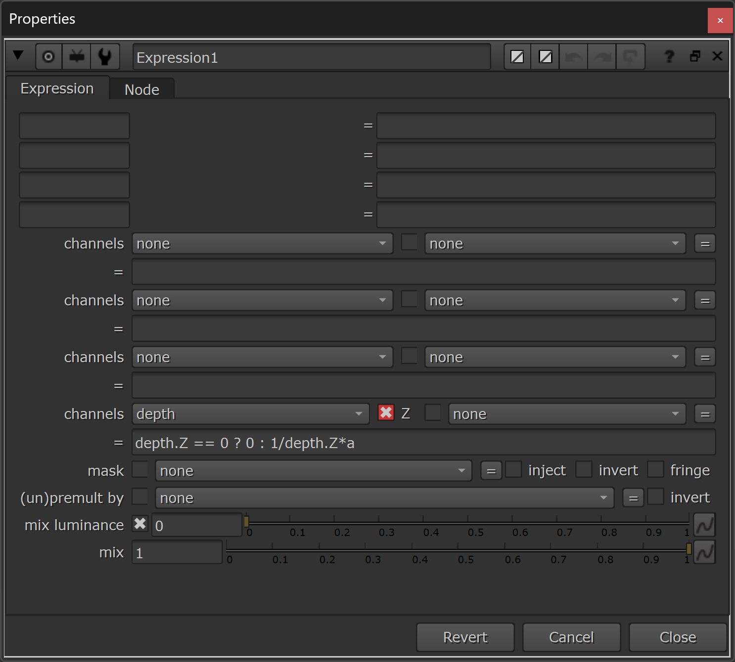

The expression to invert and premultiply the depth channel. 

The setup for outputting the particles to 2D now looks like this: 

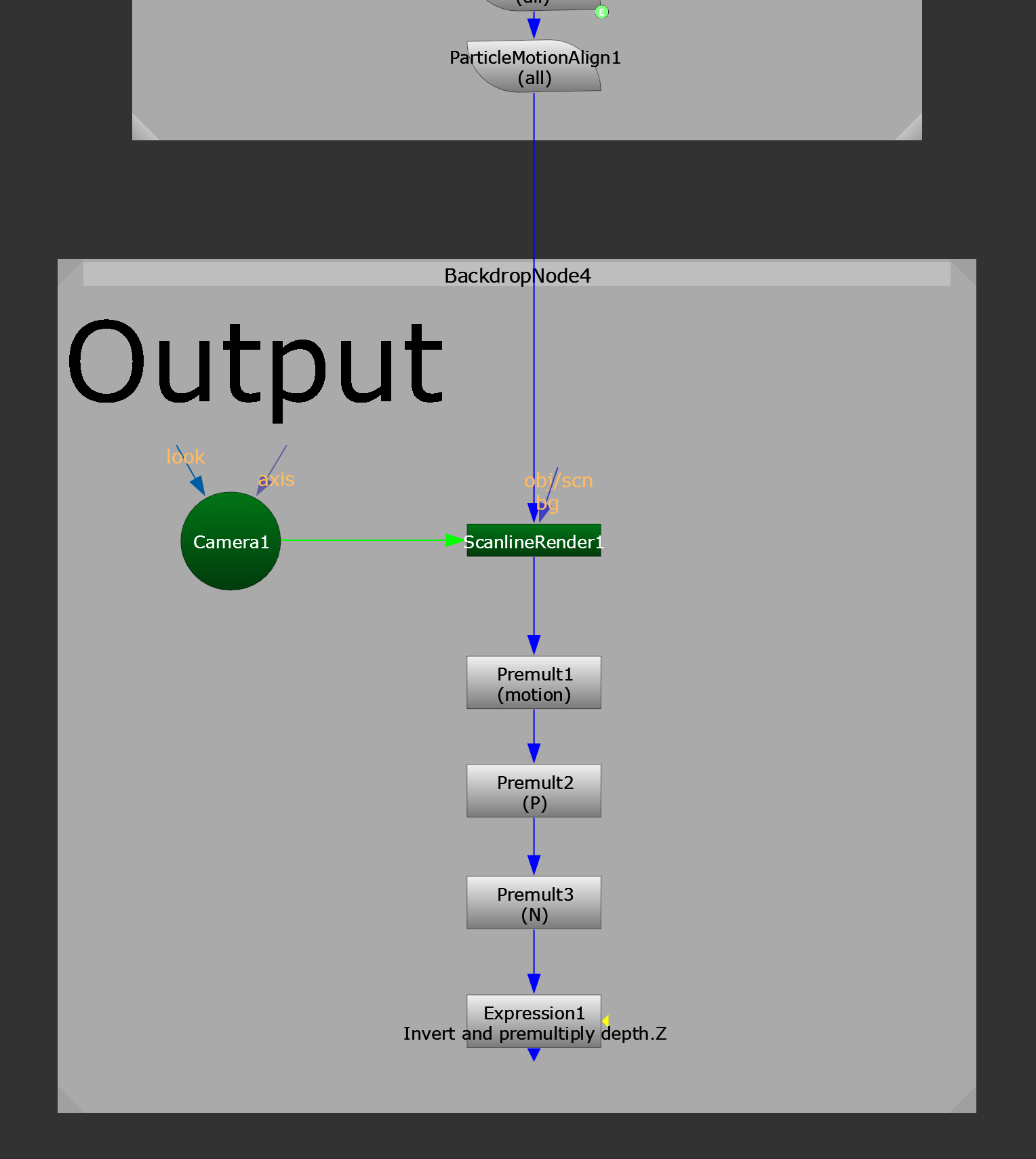
Outputting the particle insects to a 2D image sequence. 

Before we continue working on the look of the insects, let’s precomp the particles. 

Precomping The Particles

Particle systems will quickly get heavy to work with in Nuke, and so I would advise you to precomp them every time. 

Connect a Write node to the setup, set the channels to all in the Write node’s properties, and output EXR image files. 

Then, render out as many frames as you need. Earlier, we made sure that the insect animation was over-length (700 frames), so there is plenty of room to render a long frame range precomp. 

It’s a good idea to render 200-500 frames – just make sure that you have enough frames to cover the longest shots in the sequence where you’ll be using the insect element. 

I also like to make a little Switch node setup for my precomps, like this:

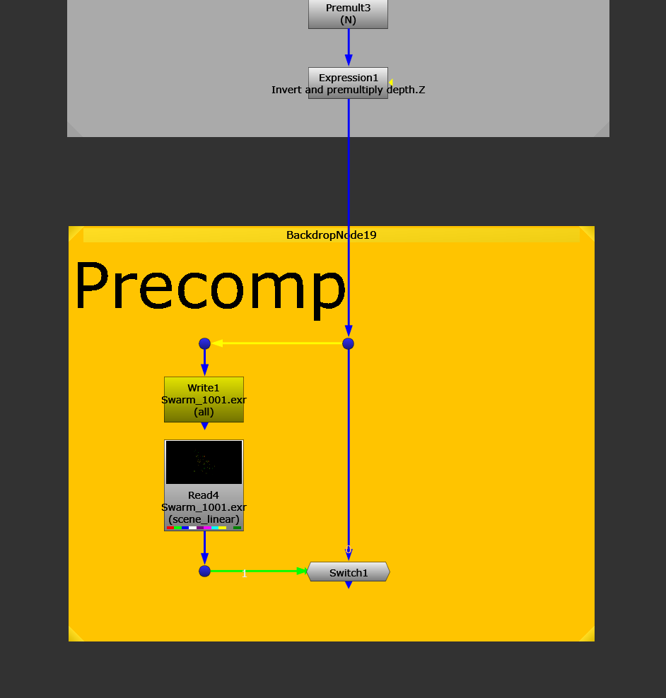
Precomping the particles. 

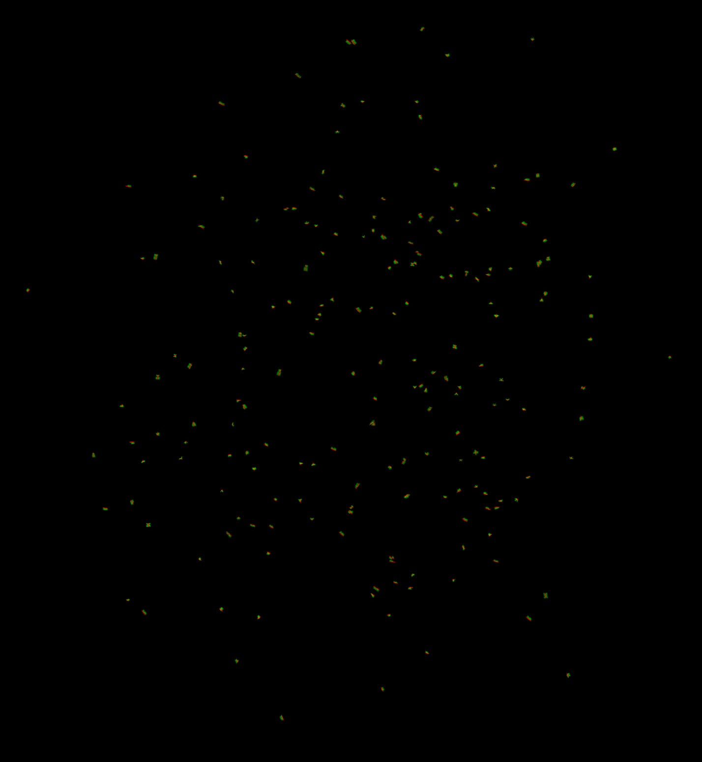
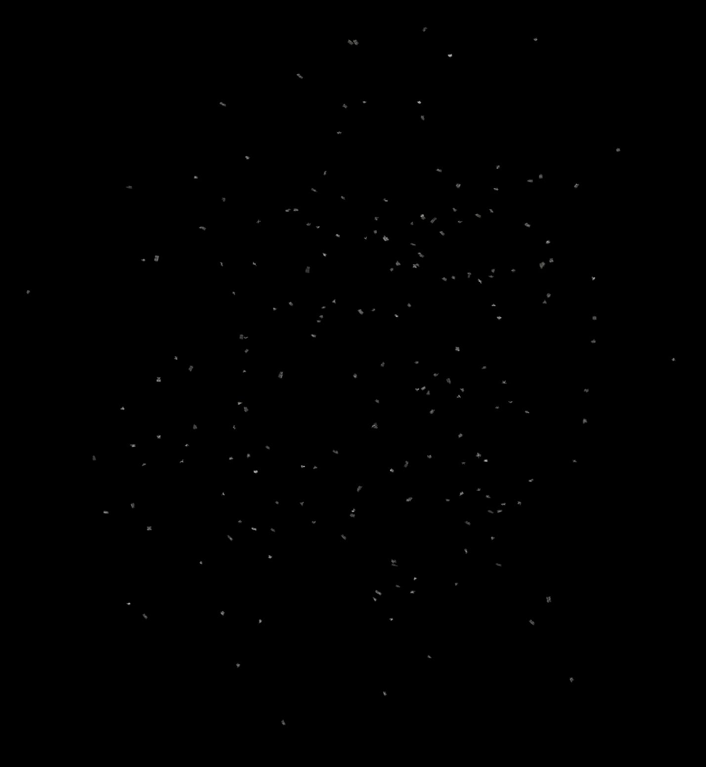
Here, I’ve only precomped a few seconds to demonstrate what the 2D output looks like in motion: 

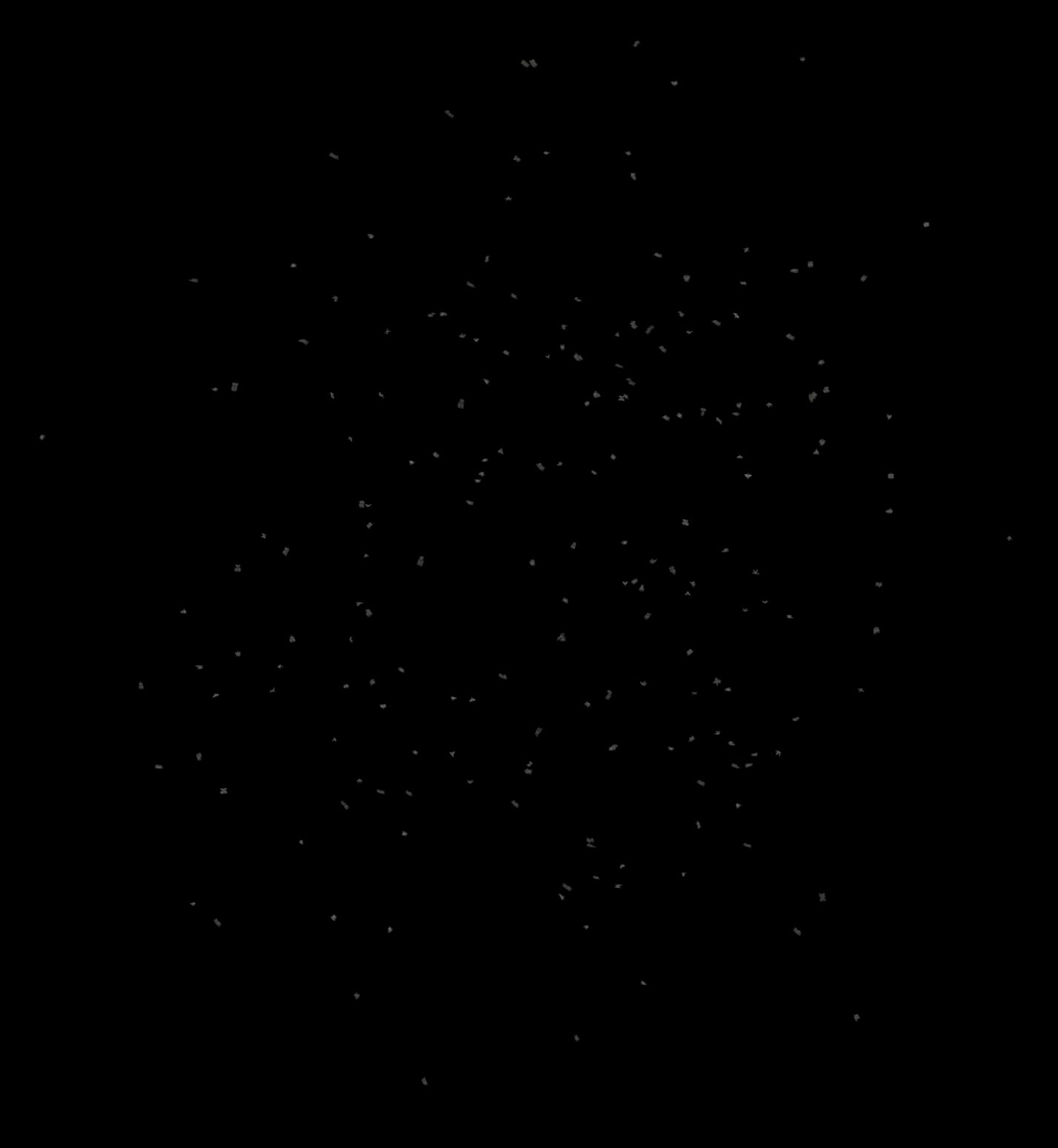
The precomped particles. 

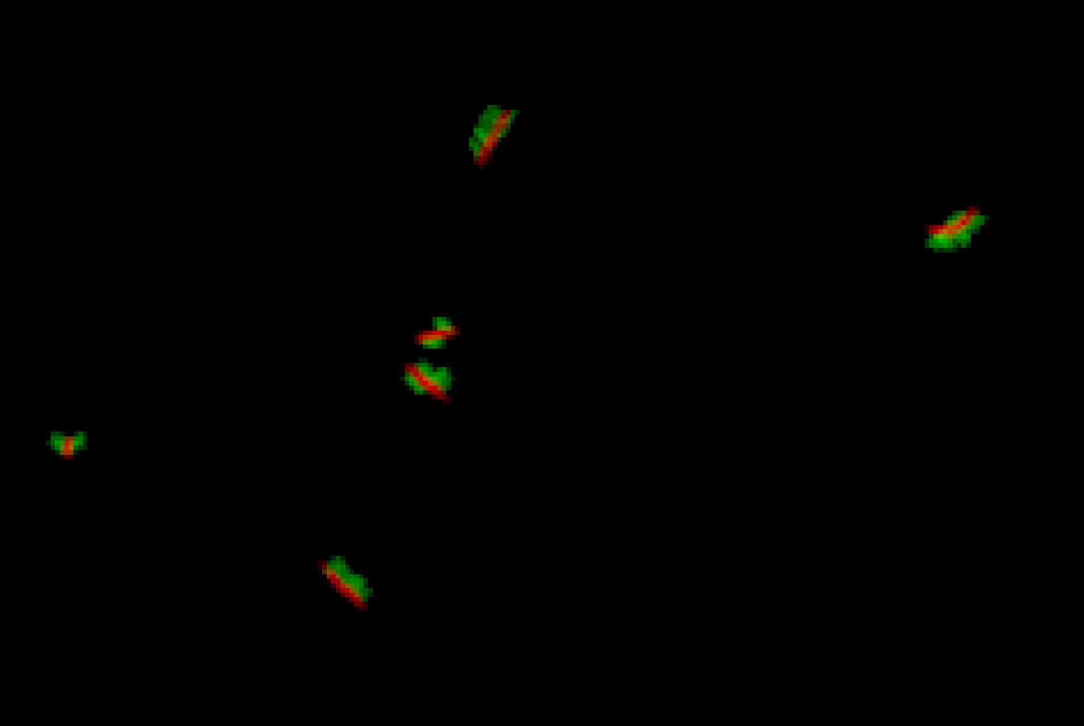
A closer look at the precomp. 

As you can see in the render, the insects have red bodies and green wings – just the way we set them up before. 

And with the additional AOVs in the EXRs, we’re now ready to adjust the look of the insects: 

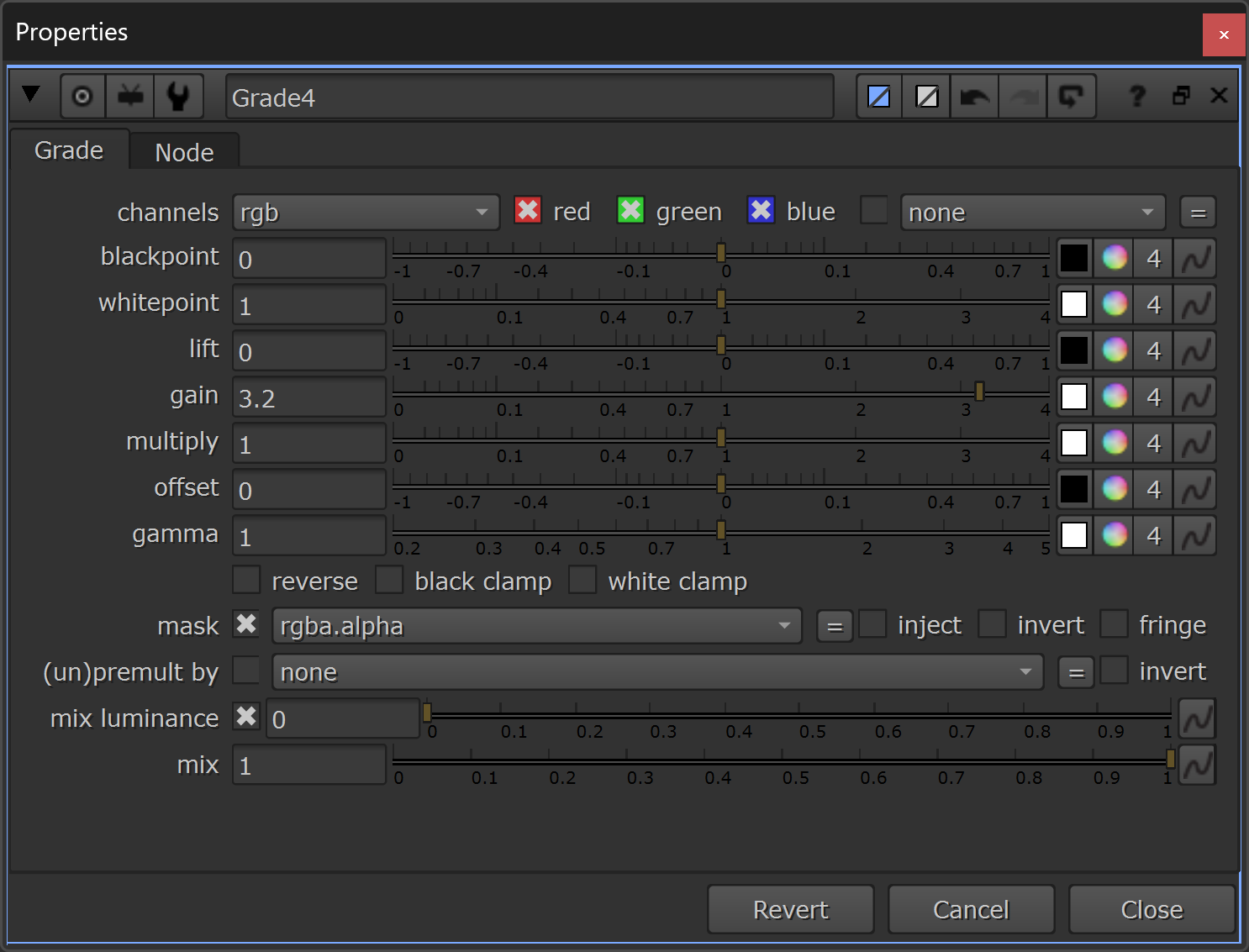
Grading The Insects

How you grade the insects will depend on your shot and sequence. 

Below, I’ve made an example setup – colouring the insects, and adding some directional lighting to them using the position and normal passes:

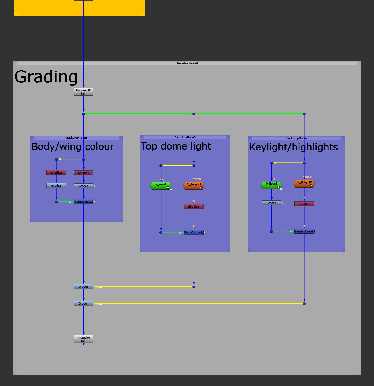
The grading setup. 

Start by unpremultiplying all of the layers with an Unpremult node set to all.

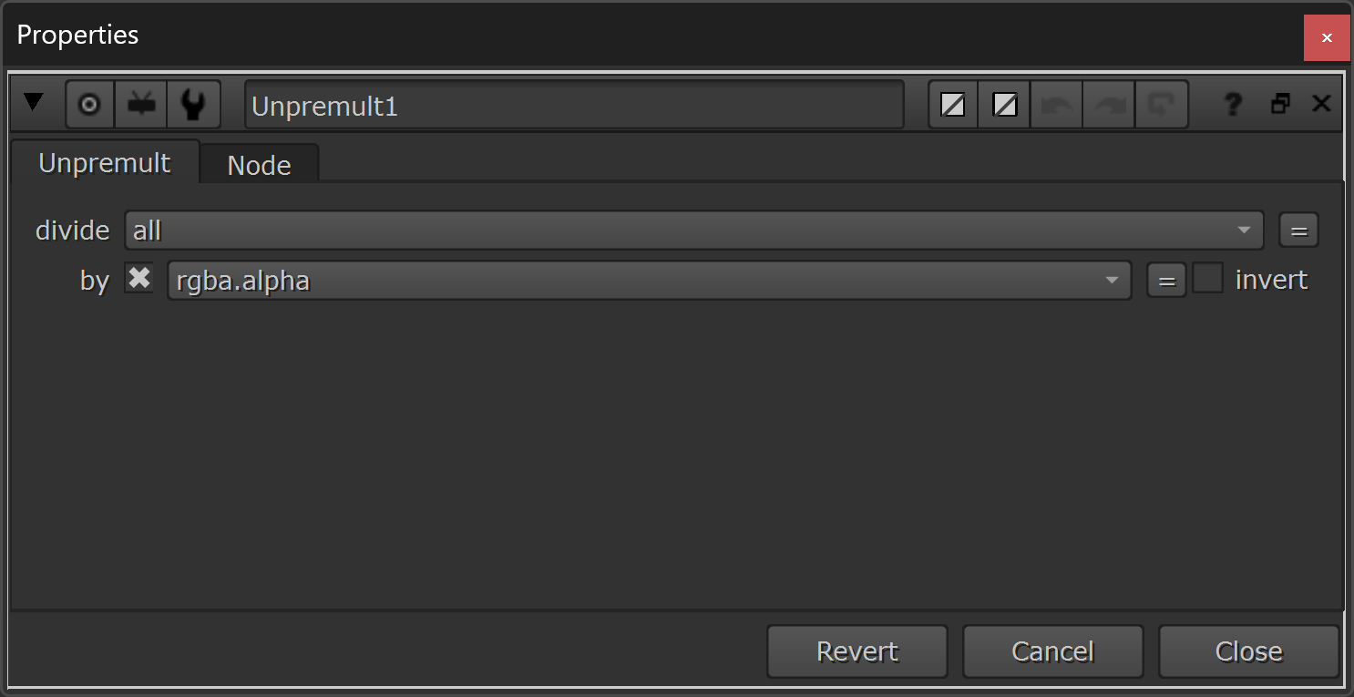
Unpremultiplying all the layers. 

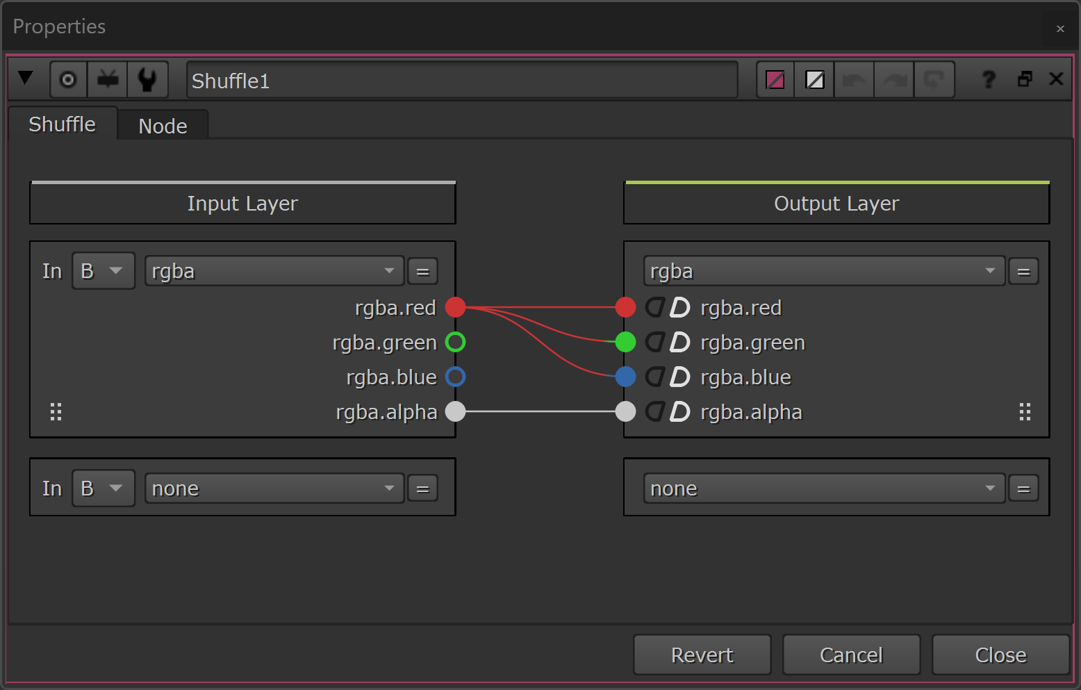
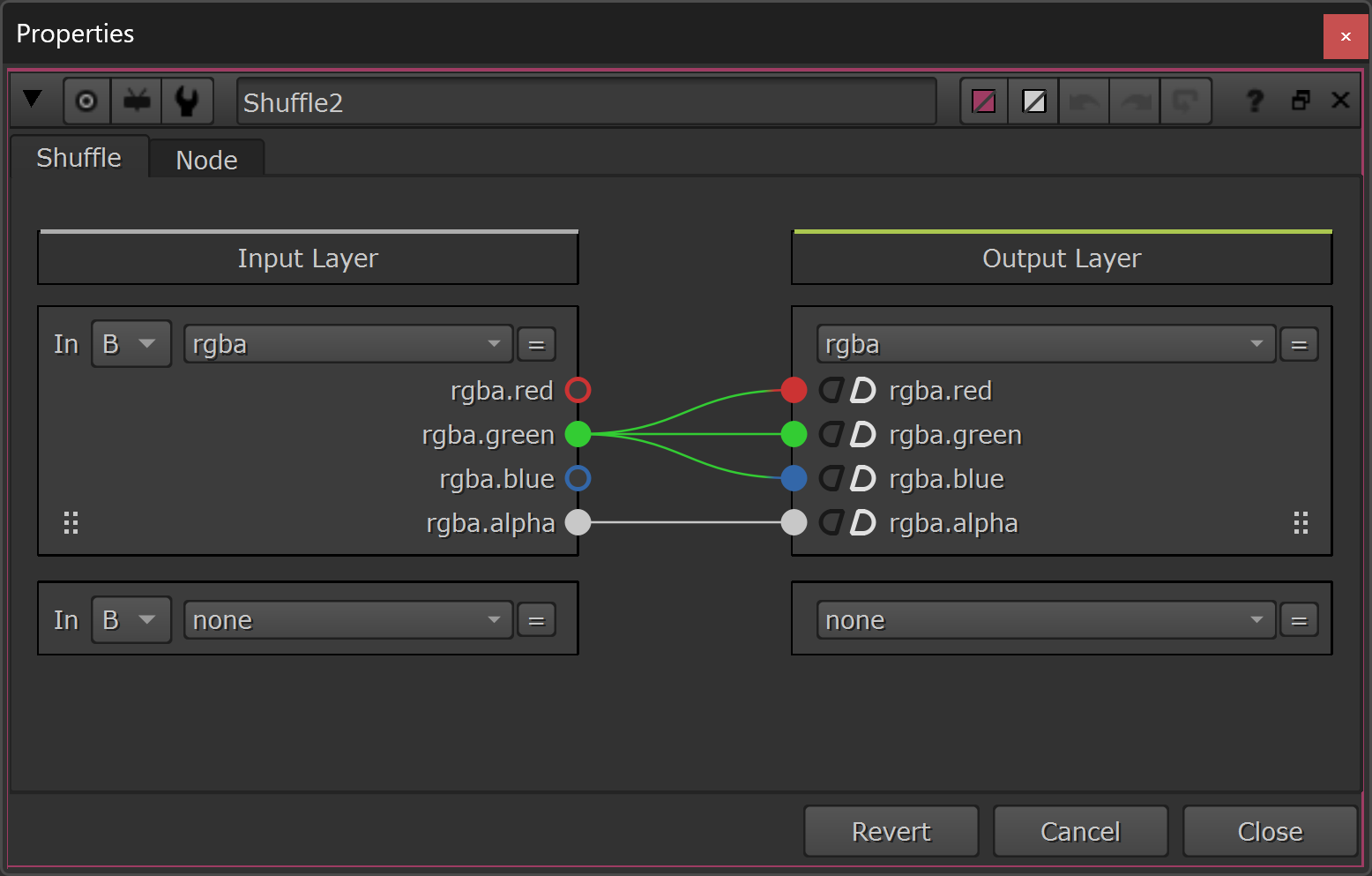
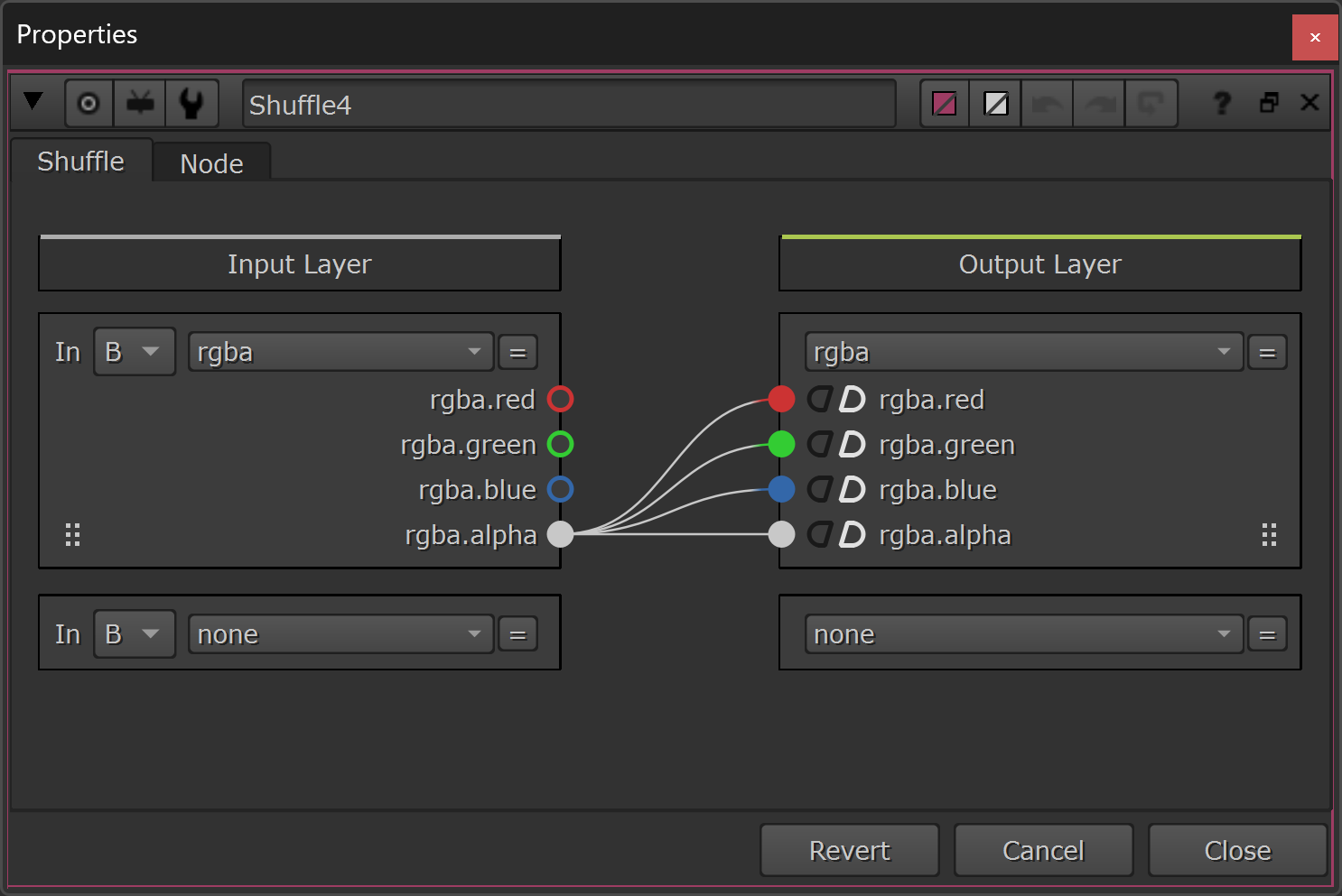
Next, shuffle out the red and green channels separately (i.e. the body and the wings of the insects), using two Shuffle nodes. (In the Body/wing colour backdrop). 

Grade each of them to taste and Merge (plus) them back together (make sure to disable the output alpha checkbox so that you don't double up the alpha). I’ve made the body a little bit darker than the wings in the example below:

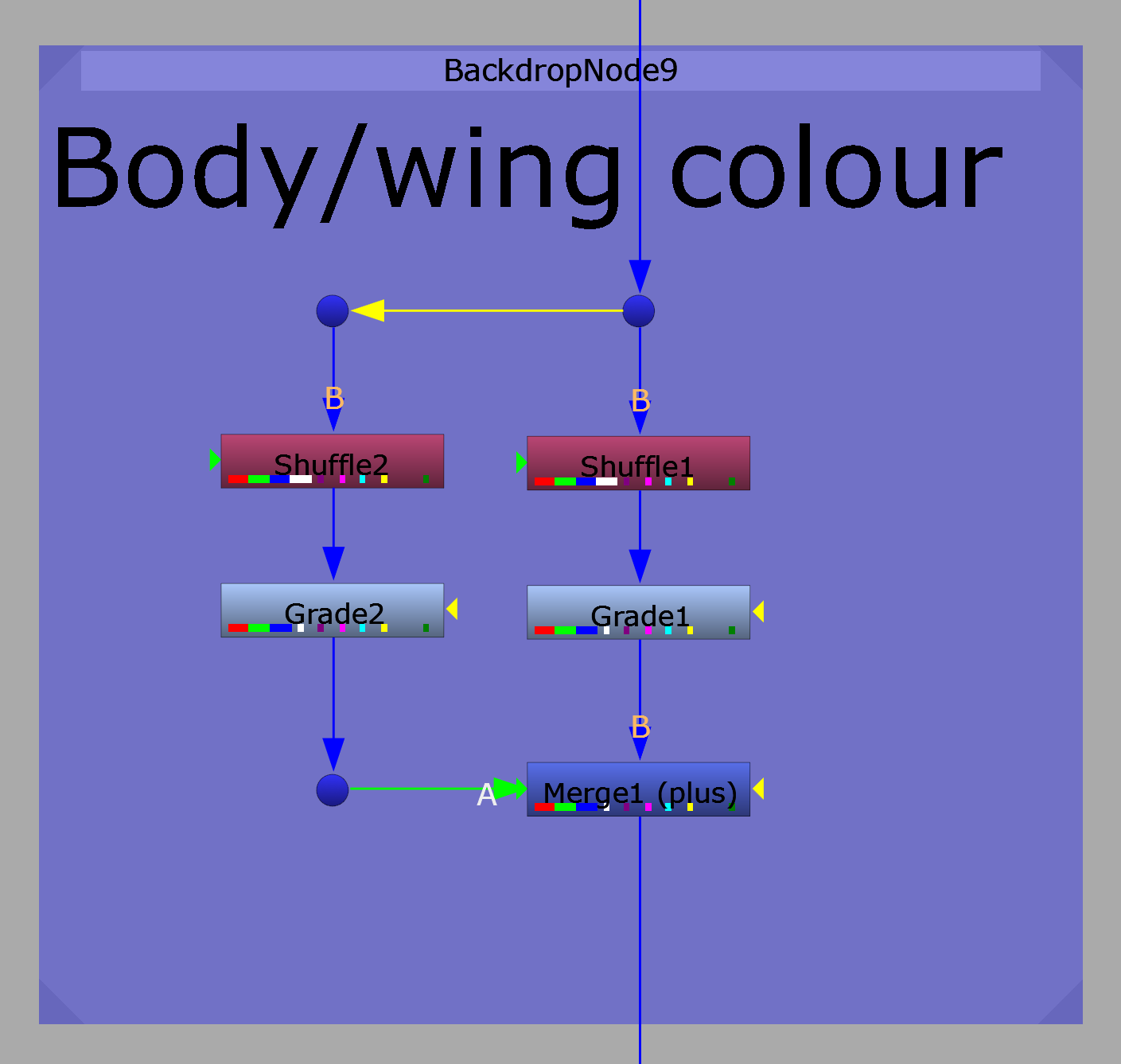
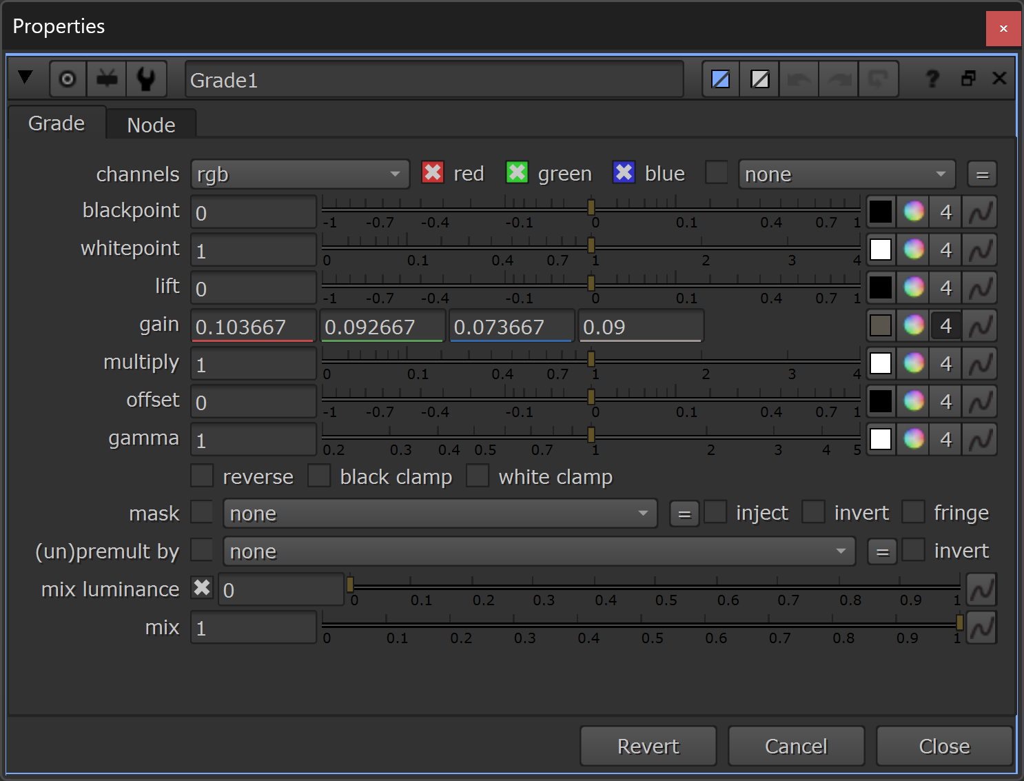
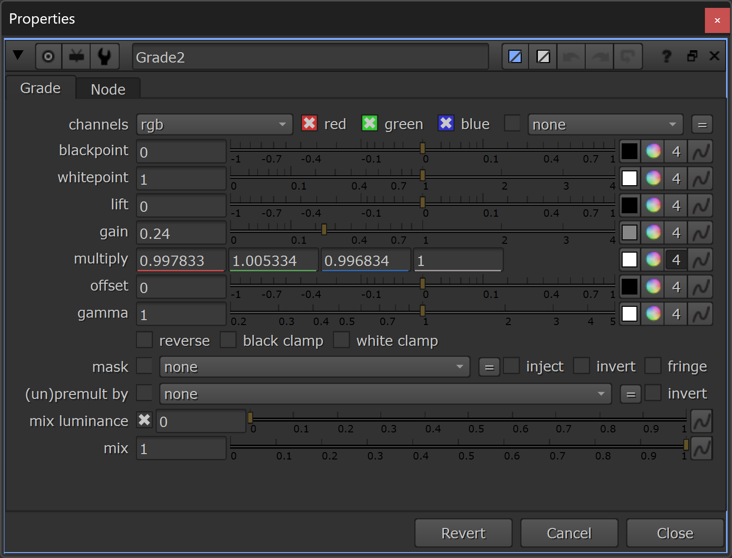
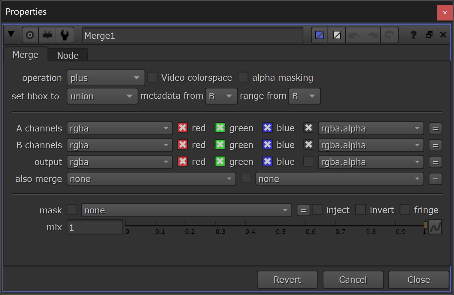
Adjusting the body/wing colour of the insects.

The base grade of the insects – basic shades of grey. 

Next, as and when needed for your shots, you can add some directional lighting and/or highlight kicks to your insects. 

Since you have both a camera and the position and normal passes, you can do a full dynamic relighting like described here: Relighting CG Renders In Nuke. 

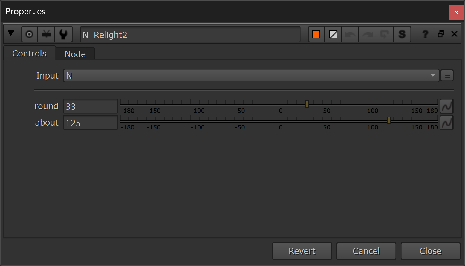
For this example, let’s do a simple relight using a ‘normal relighting’ tool, similar to the one they make in this tutorial: How To Relight Scenes in Nuke Using A Normal Pass.  

To start, let’s add a top dome light:

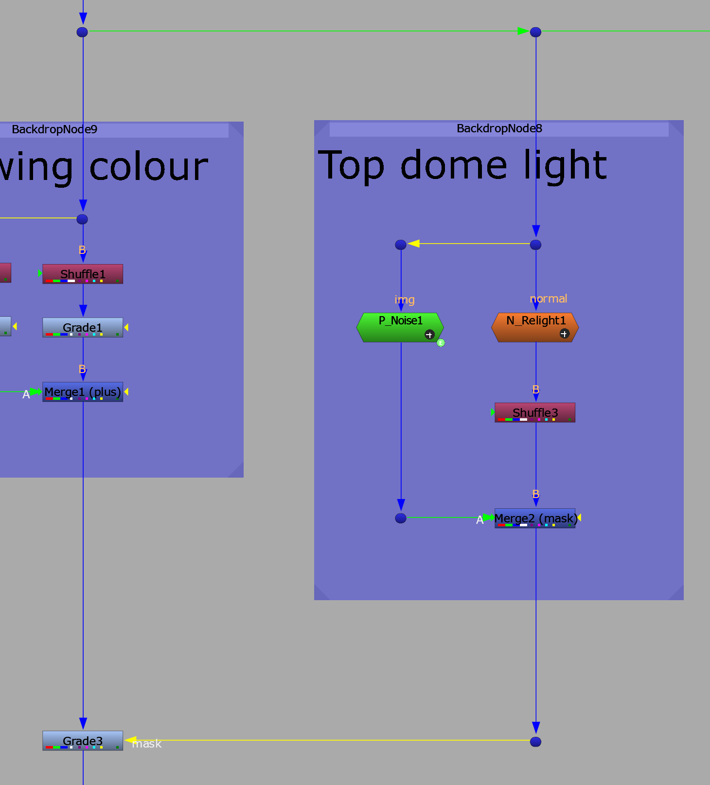
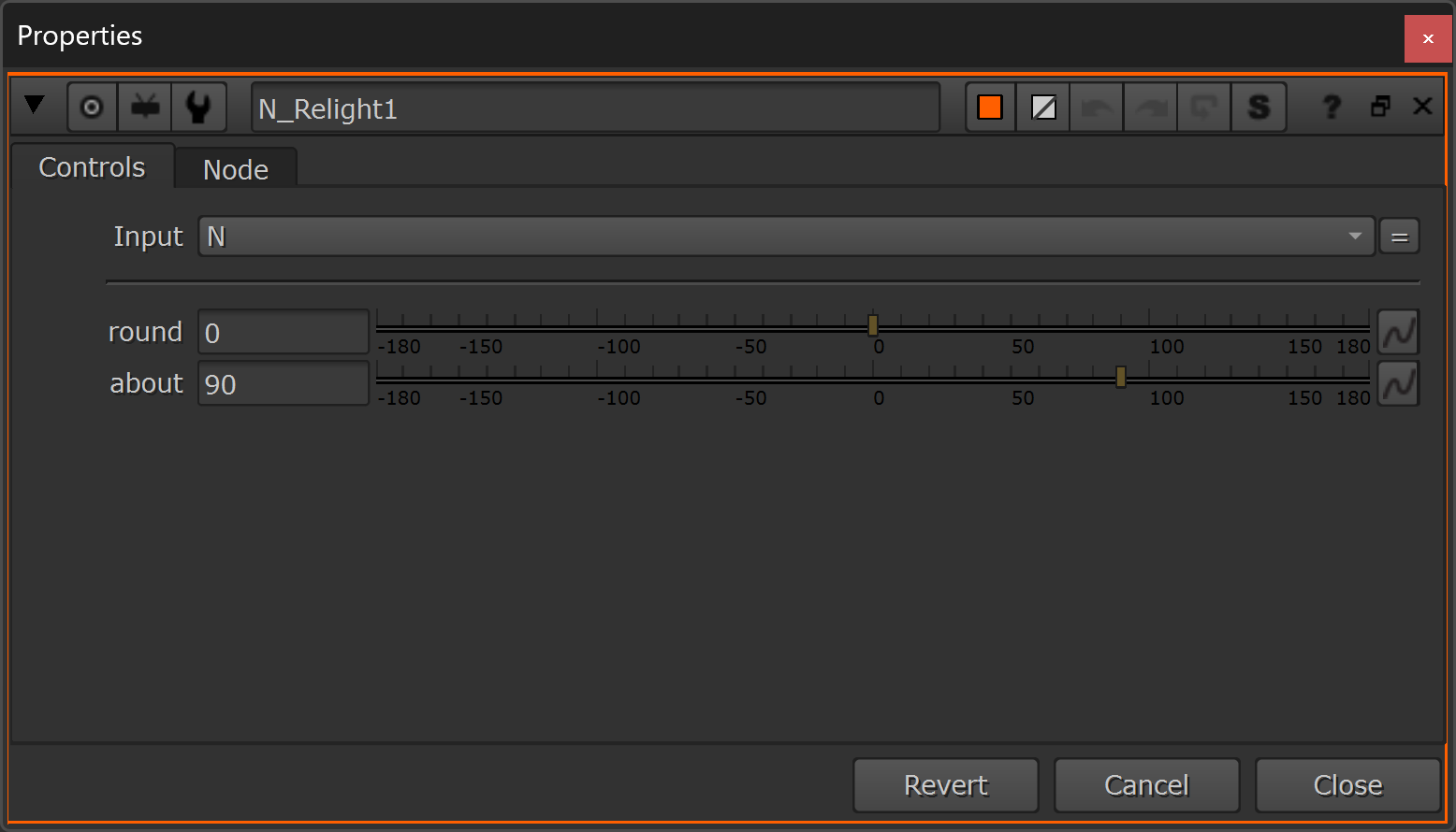
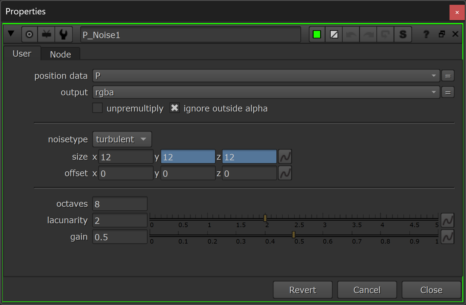
Adding a top dome light to the insects.  

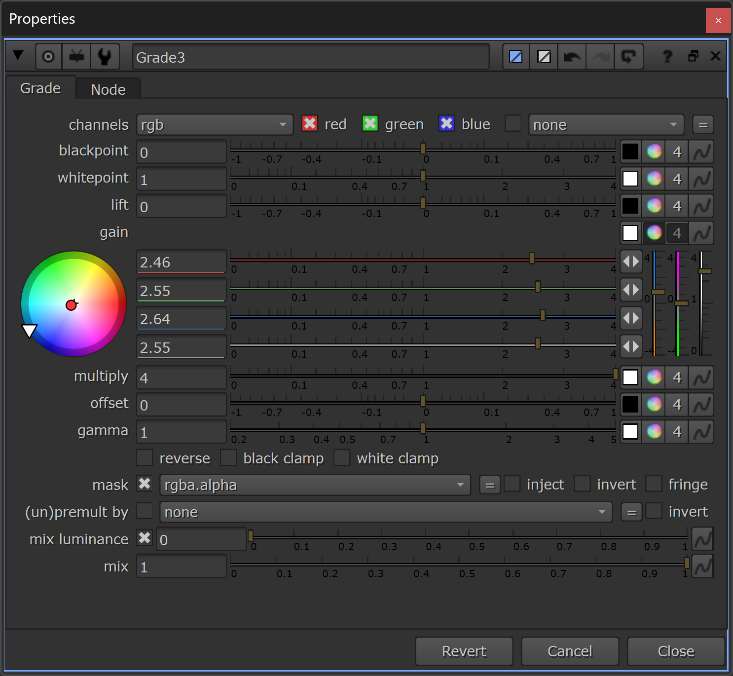
Next, let’s add a stronger kick to the light that’s hitting the insects, with a keylight/highlights: 

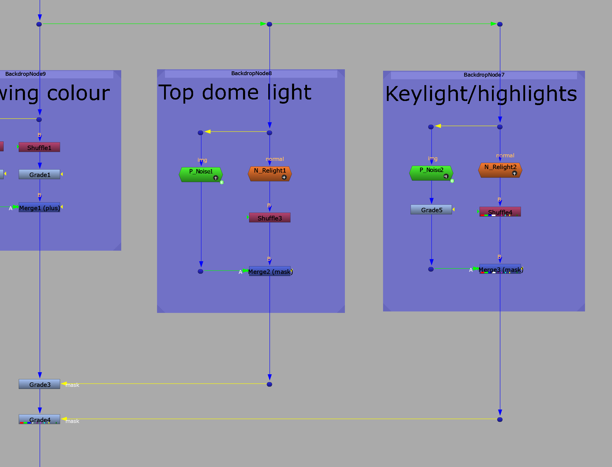
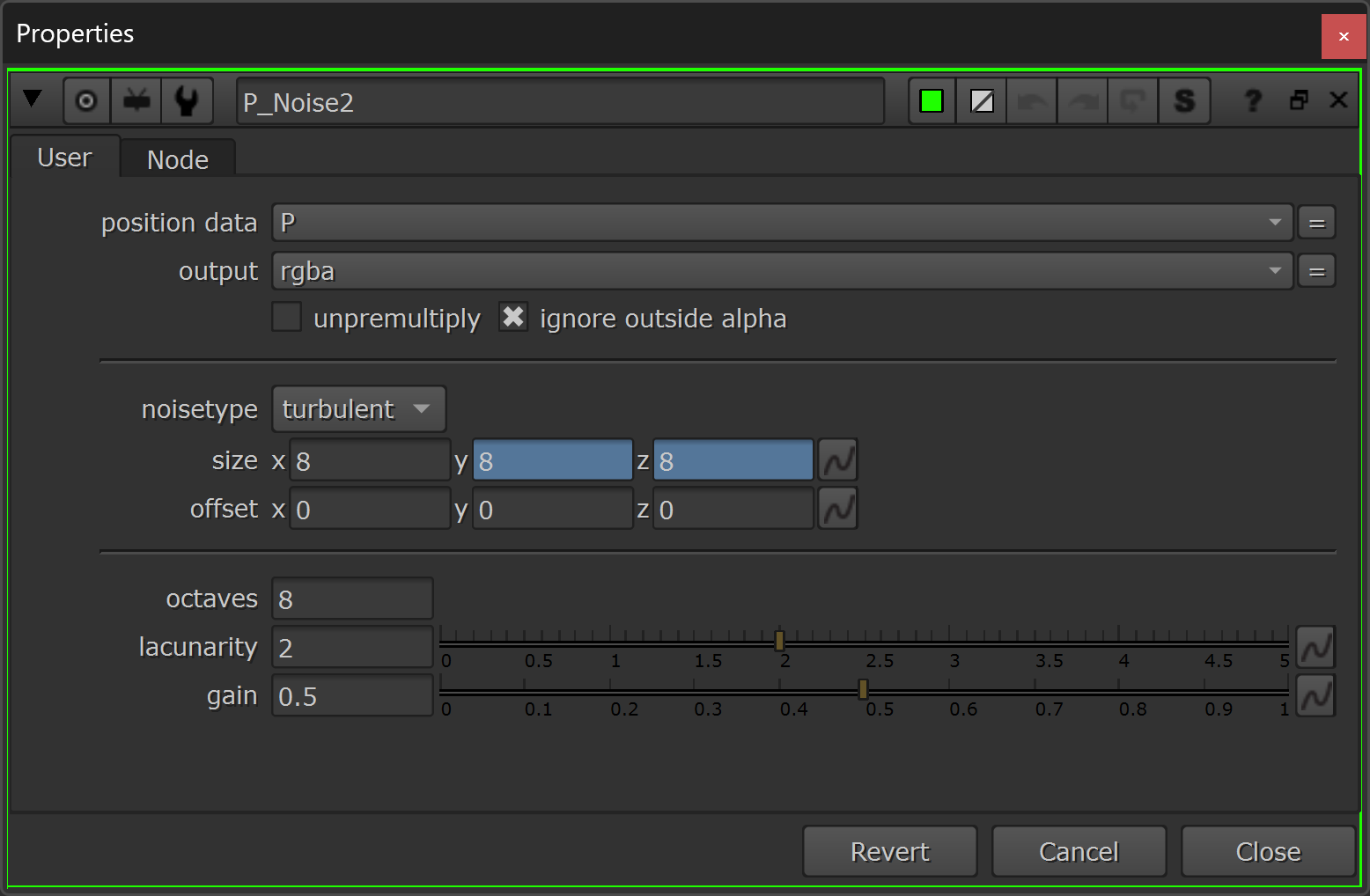
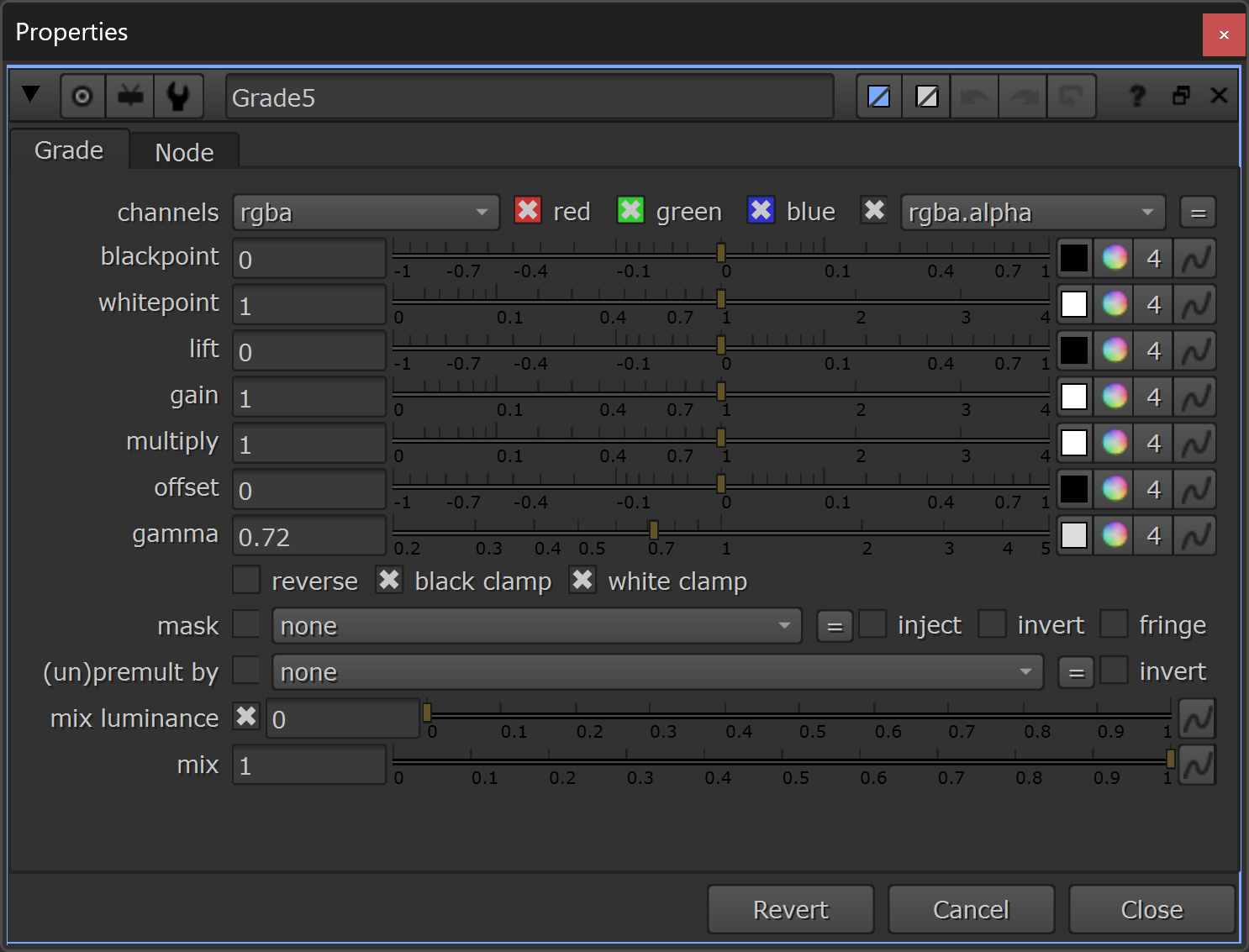
Adding a keylight/highlights to the insects. 

It’s the same exact approach as before, just different values in the nodes. And notice that we’re crunching the P_Noise matte a bit to focus on the highlights. 

Finally, premultiply all of the layers with a Premult node set to all.

Premultiplying all the layers. 

And there we have it: our graded insects: 

The final grade of the insects – with added directional lighting and highlights. 

And, in motion: 

The final render of the insects. 

Creating Variation

What we’ve made so far is just one variant. 

One element. 

To make different variations, you could go back to the particle setup and change things like: 

• The seed for the simulation. 
• The size of the insects. 
• The rate of emission (number of insects). 
• The speed of the insects.
• The turbulence/forces. 
• The geometry and/or animation of the insects.

And, you have a ton of flexibility to grade and relight the insects to your heart's content. 

Below, Companions can download the entire Nuke setup. 

I hope you found this tutorial useful. For more Nuke tips & tricks, see Nuke.